Back To Top

March 13, 2025

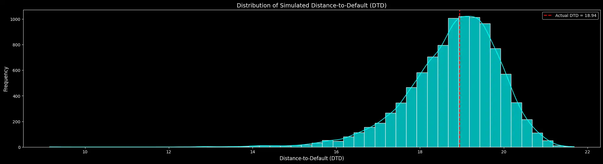
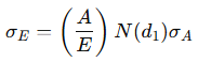
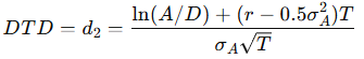
Predicting Default Risk with the Distance-to-Default Model

Using the Merton Model to estimate credit risk, simulate default probabilities, and assess financial stability

Traditional credit ratings are slow to react. The market moves faster. Investors and risk analysts need a real-time measure of financial distress — one that reflects changing market conditions, not outdated financial statements.

The Merton Model offers a solution. It treats a company’s equity as a call option on its assets, allowing us to estimate default risk directly from market prices. The key output, Distance to Default, DTD, quantifies how close a firm is to financial distress.

Use Entreprenerdly’s tool to quantify the risk of company bankruptcy in real-time:

Risk of Default Tool Demo 1 AVIF
Risk of Default Tool Demo 2 AVIF

In this guide, we’ll show:

  • How the Merton Model works in simple terms
  • How to estimate asset value and default risk using market data
  • How to apply this model in Python for real-time credit risk assessment
Figure 1. Distribution of simulated Distance to Default (DTD) based on 10,000 Monte Carlo simulations. (OPTIMIZED)

1. The Merton Model

Why Traditional Credit Risk Models Fall Short

Traditional credit risk models rely on accounting-based indicators — metrics like debt ratios, interest coverage, and credit ratings. 

The problem is that they’re backward-looking. Financial statements are updated quarterly at best, while credit ratings often lag market conditions by months. By the time distress appears in the books, the market has already reacted.

Market-Based Risk Models: A Better Approach

A firm’s stock price incorporates all available information, reacting instantly to new risks, economic shifts, and investor sentiment. 

The Merton Model leverages this by treating a company’s equity as a call option on its assets, which then allows us to estimate default risk in real time.

Instead of relying on stale financials, the Merton Model extracts risk directly from:

  • Market capitalization (E) — reflecting investor expectations
  • Stock volatility (σ_E) — capturing uncertainty in the firm’s value
  • Debt levels (D) — providing the default threshold

The Merton Model Explained

Merton’s insight: Equity is a call option on the firm’s assets.

  • Shareholders own the firm’s assets (A).
  • They must repay debt (D) at maturity (T).
  • If A > D, they keep the difference. If A < D, they default, and bondholders take over.

This follows the Black-Scholes-Merton option pricing framework, where equity value follows:

formula 1 Call option

where

formula 2 d1 and d2

Each term represents:

  • A = Asset value (firm’s total economic value)
  • D = Default point (debt obligation)
  • E = Market value of equity
  • σA = Asset volatility (uncertainty in firm’s total value)
  • r = Risk-free rate
  • N(d) = Cumulative probability from the standard normal distribution

Linking Equity Volatility to Asset Volatility

Since we observe equity (E) in the market but not assets (A) directly, we solve for A and σA using this additional equation:

formula 3 volatility equity
  • σE​ = Observed equity volatility
  • σA = Unobserved asset volatility (to be estimated)

These two equations form a nonlinear system, solved numerically to estimate A and σA.

Distance to Default: Measuring Default Risk

Once we estimate A and σA, we compute Distance to Default — a measure of how many standard deviations a firm’s assets are from default:

formula 4 DTD
  • Higher DTD → If large, the firm has a financial cushion.
  • Lower DTD → If close to zero, the firm is near default. 

2. Implementation in Python

Now, let’s apply the Merton Model in Python to estimate default risk in real time. 

Extracting Market Data for Model Inputs

To implement the model, we first need to fetch equity value, stock volatility, and debt levels. We can get this using the yfinance library.

Lets start with Debt. Different approaches to measuring debt can impact the DTD calculation and the firm’s perceived financial risk: 

  • Total Debt: Uses the total reported debt — This assumes that all obligations contribute equally to default risk.
  • Short-Term + Long-Term Debt: Adds both components directly — Gives a more detailed breakdown but assumes all reported liabilities are fully relevant.
  • Short-Term + Half of Long-Term Debt: A common approximation method — This reflects that long-term obligations may be partially refinanced or restructured before default.

Via the method argument in the function below, you can adjust for your preferred method.

When choosing the method, consider the following:

  • A higher debt value (D) leads to a lower DTD. This indicates higher default risk.
  • A lower debt value may underestimate risk. This makes the firm seem safer than it actually is.

Choosing the appropriate debt measure depends on the context of financial analysis and the firm’s borrowing structure.

				
					# Extract debt from balance sheet with multiple methods
def get_debt_from_balance_sheet(balance_sheet, info, method="STplusHalfLT", fallback=1e6):
    """
    Fetches debt based on the selected method.

    Methods:
      "TOTAL"       -> Uses the 'Total Debt' value from the balance sheet.
      "STplusHalfLT" -> Short-term debt + 0.5 * long-term debt (default).
      "STplusLT"    -> Short-term debt + long-term debt.

    If debt data is unavailable, falls back to info["totalDebt"] or a predefined fallback value.

    Inputs:
      balance_sheet = DataFrame containing balance sheet data.
      info          = Dictionary with company metadata.
      method        = Debt extraction method.
      fallback      = Default debt value if no valid data is found.

    Returns:
      debt_val = Computed debt amount.
    """

    debt_val = None
    short_debt = 0.0
    long_debt = 0.0
    total_debt = 0.0

    # Extract short-term debt
    try:
        short_debt = balance_sheet.loc["Short Term Debt"][0]
        if not np.isfinite(short_debt) or short_debt < 0:
            short_debt = 0.0
    except:
        pass

    # Extract long-term debt
    try:
        long_debt = balance_sheet.loc["Long Term Debt"][0]
        if not np.isfinite(long_debt) or long_debt < 0:
            long_debt = 0.0
    except:
        pass

    # Extract total debt
    try:
        total_debt = balance_sheet.loc["Total Debt"][0]
        if not np.isfinite(total_debt) or total_debt < 0:
            total_debt = 0.0
    except:
        pass

    # If all values are missing, fallback to info["totalDebt"]
    if short_debt == 0.0 and long_debt == 0.0 and total_debt == 0.0:
        fallback_debt = info.get("totalDebt", 0)
        if fallback_debt is not None and fallback_debt > 0:
            total_debt = fallback_debt

    # Compute debt based on the selected method
    if method.upper() == "TOTAL":
        debt_val = total_debt
    elif method.upper() == "STPLUSLT":
        debt_val = short_debt + long_debt
    else:  # Default or "STplusHalfLT"
        debt_val = short_debt + 0.5 * long_debt

    # Final check to ensure a valid debt value
    if debt_val is None or debt_val <= 0:
        debt_val = fallback

    return debt_val


Define the key parameters used in the Merton Model. 

Modify these settings to analyze different companies and market conditions. The parameters include:

  • Ticker Symbol: The stock to analyze.
  • Time Horizon (T): The forecast period in years.
  • Risk-Free Rate (r): The assumed risk-free interest rate.
  • Debt Extraction Method: The approach used to estimate total debt.
  • Volatility Calculation Period: The historical period for computing stock volatility.
				
					# Define user-controlled settings
ticker_symbol = "AAPL"  # Change this to analyze a different stock

# Model Parameters
T = 1.0           # Time horizon in years
r = 0.04          # Risk-free interest rate (annual)
debt_method = "STplusHalfLT"  # Options: "TOTAL", "STplusHalfLT", "STplusLT"
debt_factor = 1.0  # Scaling factor applied to debt

# Volatility Calculation
historical_period = "1y"  # Period used to compute equity volatility (e.g., "1y", "2y", "6mo")
annualization_factor = 252  # Annualization factor for daily stock returns


Next, we get:

  • Stock price (regularMarketPrice)
  • Shares outstanding (sharesOutstanding)
  • Historical stock prices (for volatility estimation)

The stock’s market cap (E) is calculated from price × shares outstanding. Equity volatility (σE) is estimated from historical log returns, annualized over 252 trading days.

Prev Post

CBOE BZX Files to Trade Franklin Templeton XRP ETF

Next Post

Estimating Bid-Ask Spreads Using OHLC Prices

post-bars
Mail Icon

Newsletter

Get Every Weekly Update & Insights

[mc4wp_form id=]

Leave a Comment