Experience the Future of Intelligent Investing Today
Back To Top
Experience the Future of Intelligent Investing Today
Most traders underestimate how much bid-ask spreads eat into their profits. Even small spreads can significantly impact execution costs, especially in low-liquidity markets.
Yet, accurately measuring spreads isn’t straightforward — especially when relying on open, high, low, and close (OHLC) prices instead of full order book data.
A more accurate approach is outlined in the work of Ardia, Guidotti, and Kroencke (2024), who propose an estimator that improves spread measurement using Generalized Method of Moments and OHLC price transformations.
This method corrects for price discreteness and minimizes estimation variance. Unlike older models, it adapts to market conditions in real-time. It’s a powerful tool for traders, quants, and financial researchers.

In this article, we’ll break down the problem, explain the math behind the estimator, and show how to implement it in Python.
Finally, we’ll analyze real-world bid-ask spreads for AAPL stock to get insights into transaction costs and liquidity.
Traditional methods rely on assumptions that often do not hold in real markets. This leads to biased and inconsistent estimates.
One of the most cited models, the Roll estimator, derives the spread from the negative serial covariance of price changes:
Ct is the closing price at time t. This method assumes:
However, in real markets:
To reduce variance, Corwin & Schultz (2012) proposed an estimator using high and low prices:
B represents the variance of log high-low price ratios. This model assumes:
Both assumptions fail in markets with price jumps and volatility clustering, which makes it an unreliable estimator.
An improvement by Abdi & Ranaldo (2017) integrates closing, high, and low prices:
where ηt is the mid-price. While this reduces bias, it still fails to fully account for discrete price observations. This leads to inaccuracies in low-trading-frequency markets.
Ardia et al. (2024) address these limitations by incorporating all OHLC price observations.
Their key innovation uses moment conditions to isolate bid-ask spread effects while controlling for fundamental price variations.
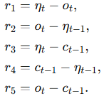
The approach defines multiple log-returns based on OHLC prices:


ot, ct, Ht, Lt are log-transformed open, close, high, and low prices.
A key correction is introduced via an indicator for price variation, which adjusts for cases where prices remain unchanged:

The method avoids overestimating spreads when price changes are minimal to address a key weakness in prior models.
This estimator improves bid-ask spread measurement by leveraging OHLC prices and a rolling window to track liquidity trends dynamically.
The spread estimate is computed as:

ηt is the midpoint log-price, and τt accounts for price variation.
Key advantages:
This method reduces bias and improves precisio. It outperforms traditional estimators, especially in low-liquidity markets.
The following implementation borrows its core logic from the original repository by Ardia et al. (2024).

Newsletter