Portfolio optimization across multiple factors - Dividends, Returns, Volatility, CVaR, and more
Multi-objective Portfolio optimization considers multiple objectives simultaneously, such as maximizing returns, minimizing risk, and enhancing diversification, to build a portfolio that aligns with the investor’s goals across multiple factors.
In this article, we’ll optimize a portfolio based on multiple objectives, such as dividend yields, maximise returns, maximise Sharpe ratio, and more.
We offer end-to-end implementation code using Google Colab Notebook. Additionally, Entreprenerdly’s automated portfolio optimization tool is available here.
The tool allows investors to directly implement various portfolio optimization techniques to best suit their individual risk preferences and return expectations.

We’ll discuss and implement the following concepts:
- Defining Objectives Function
- Returns, Risk, Dividends, etc
- Retrieving weights
- Parameters Grid Search
- Rebalancing Periods
- Best Possible Portfolio
- Assessing Portfolio Performance
- Performance Attribution
- Allocation, Selection, Interaction Effect
- Sector Allocation Risks
- Rolling Performance Metrics
2. Multi-Objective Portfolio Optimization
2.1 Approach and Methodology
The methodology involves defining various objectives and constraints to optimize the portfolio. The core approach in optimizing a multi-objective portfolio revolves around balancing several investment goals simultaneously.
1. Define Objectives and Constraints
Each objective represents a specific goal we want the portfolio to achieve, such as maximizing returns or minimizing risk. Constraints ensure the portfolio remains realistic and feasible, like ensuring the sum of asset weights equals one.
2. Formulate the Objective Function
We create a single objective function that incorporates all the individual objectives. The function quantifies how well the portfolio meets each goal. For instance, if we want to maximize returns and minimize risk, the objective function could look like this:
Here, ∑(wi⋅μi) represents the portfolio’s expected return, and sqrt{wT⋅Σ⋅w} represents the portfolio’s risk.
3. Weighting the Objectives
Not all objectives are equally important. We assign weights to each objective based on their relative importance. This step helps prioritize certain goals over others to reflect the investor’s preferences.
4. Optimization Algorithm
We use Sequential Least Squares Programming (SLSQP) to find the optimal set of asset weights. The algorithm iteratively adjusts the weights to minimize or maximize the objective function while adhering to the constraints. The goal is to find the set of weights that best achieves the defined objectives.
5. Periodic Rebalancing
Portfolios are rebalanced periodically to ensure they stay aligned with the original objectives. During rebalancing, we adjust the asset weights to account for market changes and shifts in the investor’s goals.
2.2 The Objectives to Optimize
The following objectives can be customized by setting them to 'true' or 'false' in the implementation code, based on whether the user wants to include them in the optimization process.
Maximize Return
We aim to maximize the expected return of the portfolio by calculating the weighted sum of mean returns. The objective value is adjusted by subtracting this weighted sum:
where wi represents the weight of asset i and μi is the expected return of asset i.
Minimize Risk
To minimize risk, we consider the portfolio’s volatility (standard deviation). This is achieved by adding the portfolio’s standard deviation to the objective value:
Σ is the covariance matrix of asset returns.
Maximize Sharpe Ratio
The Sharpe ratio measures risk-adjusted return. We calculate it and subtract it from the objective value:
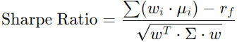
where rf is the risk-free rate.
Maximize Diversification
Diversification is assessed by comparing the weighted sum of individual asset volatilities to the portfolio’s volatility. This ratio is subtracted from the objective value:
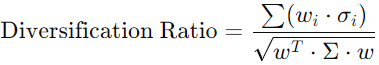
Other measures, such as HHI (Herfindahl-Hirschman Index), could be used instead.
Minimize CVaR
Conditional Value at Risk (CVaR) represents the expected loss in the worst-case scenario. The objective value is increased by adding the 5th percentile of portfolio returns:
Minimize Transaction Costs
To account for transaction costs, we assume a previous portfolio with equal weights. The costs are calculated and added to the objective value:
where wi,prev is the previous weight of asset i.
Maximize Dividend Yield
We maximize dividend yield by subtracting the weighted sum of dividend yields from the objective value:
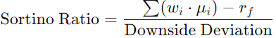
Maximize Sortino Ratio
The Sortino ratio focuses on downside risk. It is calculated and subtracted from the objective value:
Maximize Upside Potential Ratio
This ratio compares the mean of positive returns to downside risk. The ratio is subtracted from the objective value:

Minimize Beta
Beta measures the portfolio’s volatility relative to the market. We add the portfolio beta to the objective value:
2.4 Python Implementation
2.4.1 Core Functions
Lets discuss now the essential functions required for multi-objective portfolio optimization using Python. These functions facilitate data download, metric calculations, optimization, and visualization:
Dynamic Data Alignment: In
portfolio_beta, the function dynamically aligns the portfolio’s returns with the benchmark returns usingalign. This ensures both datasets are on the same date range, preventing misalignment issues that could skew results.Handling Missing Data: The
calculate_metricsfunction drops any rows with missing data (dropna). This is needed as financial data often contains gaps due to holidays.Multi-Objective Optimization: The
multi_objective_functionallows the inclusion or exclusion of various objectives such as maximizing return, minimizing risk, or maximizing dividend yield. Each objective modifies theobj_value, balancing trade-offs according to user-defined priorities.Periodic Rebalancing: The
rebalance_portfoliofunction ensures that the portfolio stays aligned with the defined objectives by adjusting the weights periodically as market conditions change.Realistic Constraints: The
optimize_portfoliofunction includes constraints to ensure that the sum of weights equals 1 and that all weights are between 0 and 1.
					import yfinance as yf
import numpy as np
import pandas as pd
import matplotlib.pyplot as plt
from scipy.optimize import minimize
from pypfopt import risk_models, expected_returns
import json

# Function to download adjusted close prices for given tickers
def download_data(tickers, start, end):
    return yf.download(tickers, start=start, end=end)['Adj Close']

# Function to calculate returns, mean returns, and covariance matrix
def calculate_metrics(data):
    returns = data.pct_change().dropna()  # Calculate daily returns
    mean_returns = expected_returns.mean_historical_return(data)  # Calculate mean returns
    cov_matrix = risk_models.sample_cov(data)  # Calculate covariance matrix
    return returns, mean_returns, cov_matrix

# Function to get dividend yields for given tickers
def get_dividend_yields(tickers):
    dividend_yields = {}
    for ticker in tickers:
        stock = yf.Ticker(ticker)
        info = stock.info
        # Get dividend yield or set to 0 if not available
        dividend_yield = info.get('dividendYield') or info.get('trailingAnnualDividendYield', 0)
        if dividend_yield is None:
            dividend_yield = 0
        dividend_yields[ticker] = dividend_yield
    return pd.Series(dividend_yields)

# Function to calculate portfolio beta
def portfolio_beta(weights, returns, benchmark_returns):
    aligned_returns, aligned_benchmark = returns.align(benchmark_returns, join='inner', axis=0)
    cov_matrix = np.cov(aligned_returns.T, aligned_benchmark)
    beta = cov_matrix[:-1, -1] / np.var(aligned_benchmark)
    return np.sum(weights * beta)

# Function to calculate Sortino ratio
def sortino_ratio(weights, returns, risk_free_rate=0.01):
    portfolio_return = np.dot(weights, returns.mean())
    downside_returns = np.minimum(returns - risk_free_rate, 0)
    downside_deviation = np.sqrt(np.mean(downside_returns ** 2))
    return (portfolio_return - risk_free_rate) / downside_deviation

# Function to calculate Upside Potential Ratio
def upside_potential_ratio(weights, returns, risk_free_rate=0.01):
    portfolio_return = np.dot(weights, returns.mean())
    upside_returns = np.maximum(returns - risk_free_rate, 0)
    downside_returns = np.minimum(returns - risk_free_rate, 0)
    downside_deviation = np.sqrt(np.mean(downside_returns ** 2))
    upside_potential = np.mean(upside_returns)
    return upside_potential / downside_deviation

# Multi-objective function for portfolio optimization
def multi_objective_function(weights, mean_returns, cov_matrix, dividend_yields, benchmark_returns, risk_free_rate=0.01):
    obj_value = 0  # Initialize the objective value to 0
    if maximize_return:
        # If we want to maximize return, subtract the weighted sum of mean returns from the objective value
        obj_value -= np.dot(weights, mean_returns)  # Maximize return
    if minimize_risk:
        # If we want to minimize risk, add the portfolio volatility (standard deviation) to the objective value
        obj_value += np.sqrt(np.dot(weights.T, np.dot(cov_matrix, weights)))  # Minimize risk
    if maximize_sharpe:
        # If we want to maximize the Sharpe ratio, calculate it and subtract from the objective value
        portfolio_return = np.dot(weights, mean_returns)  # Expected portfolio return
        portfolio_volatility = np.sqrt(np.dot(weights.T, np.dot(cov_matrix, weights)))  # Portfolio volatility
        sharpe_ratio = (portfolio_return - risk_free_rate) / portfolio_volatility  # Sharpe ratio calculation
        obj_value -= sharpe_ratio  # Maximize Sharpe ratio
    if maximize_diversification:
        # If we want to maximize diversification, calculate the diversification ratio and subtract it from the objective value
        w_vol = np.dot(weights.T, np.sqrt(np.diag(cov_matrix)))  # Weighted volatilities of individual assets
        p_vol = np.sqrt(np.dot(weights.T, np.dot(cov_matrix, weights)))  # Portfolio volatility
        diversification_ratio = w_vol / p_vol  # Diversification ratio calculation
        obj_value -= diversification_ratio  # Maximize diversification
    if minimize_cvar:
        # If we want to minimize Conditional Value at Risk (CVaR), calculate it and add to the objective value
        cvar = np.percentile(np.dot(returns.values, weights), 5)  # CVaR calculation
        obj_value += cvar  # Minimize CVaR
    if minimize_transaction_costs:
        # If we want to minimize transaction costs, calculate them and add to the objective value
        prev_weights = np.ones(len(weights)) / len(weights)  # Assume equal weights previously
        transaction_costs = np.sum(np.abs(weights - prev_weights)) * 0.001  # Assume 0.1% cost for transactions
        obj_value += transaction_costs  # Minimize transaction costs
    if maximize_dividend_yield:
        # If we want to maximize dividend yield, subtract the weighted sum of dividend yields from the objective value
        obj_value -= np.dot(weights, dividend_yields)  # Maximize dividend yield
    if maximize_sortino:
        # If we want to maximize the Sortino ratio, calculate it and subtract from the objective value
        obj_value -= sortino_ratio(weights, returns, risk_free_rate)  # Maximize Sortino ratio
    if maximize_upside_potential:
        # If we want to maximize the Upside Potential Ratio, calculate it and subtract from the objective value
        obj_value -= upside_potential_ratio(weights, returns, risk_free_rate)  # Maximize Upside Potential Ratio
    if minimize_beta:
        # If we want to minimize beta, calculate it and add to the objective value
        obj_value += portfolio_beta(weights, returns, benchmark_returns)  # Minimize Beta
    return obj_value  # Return the final objective value


# Function to optimize portfolio based on given metrics
def optimize_portfolio(mean_returns, cov_matrix, dividend_yields, benchmark_returns):
    num_assets = len(mean_returns)
    init_guess = num_assets * [1. / num_assets,]  # Initial guess for weights
    constraints = ({'type': 'eq', 'fun': lambda x: np.sum(x) - 1}, {'type': 'ineq', 'fun': lambda x: x})  # Constraints
    bounds = [(0, 1) for _ in range(num_assets)]  # Bounds for weights
    result = minimize(multi_objective_function, init_guess, args=(mean_returns, cov_matrix, dividend_yields, benchmark_returns),
                      method='SLSQP', bounds=bounds, constraints=constraints)
    return result.x

# Function to calculate cumulative returns
def calculate_cumulative_returns(returns, weights):
    portfolio_returns = returns.dot(weights)
    return (1 + portfolio_returns).cumprod()

# Function to plot cumulative returns
def plot_results(portfolio_cumulative, sp500_cumulative, equal_weighted_cumulative):
    plt.figure(figsize=(10, 6))
    plt.plot(portfolio_cumulative, label='Multi-Objective Optimization Portfolio')
    plt.plot(sp500_cumulative, label='S&P 500')
    plt.plot(equal_weighted_cumulative, label='Equal Weighted Portfolio')
    plt.xlabel('Date')
    plt.ylabel('Cumulative Returns')
    plt.title('Cumulative Returns Over Time')
    plt.legend()
    plt.show()

# Function to rebalance portfolio periodically
def rebalance_portfolio(data, tickers, rebalance_period):
    rebalanced_weights = []
    dates = pd.date_range(start=data.index[0], end=data.index[-1], freq=f'{rebalance_period}M')
    for date in dates:
        if date in data.index:
            subset_data = data[:date]  # Data up to the current date
            returns, mean_returns, cov_matrix = calculate_metrics(subset_data)
            benchmark_returns = benchmark_data[:date].pct_change().dropna()
            dividend_yields = get_dividend_yields(tickers)
            weights = optimize_portfolio(mean_returns, cov_matrix, dividend_yields, benchmark_returns)
            rebalanced_weights.append((date, weights))
    return rebalanced_weights
2.4.2 Main Execution
We execute now the main functions, considering the following steps:
Define Global Objectives: We set variables, to true or false, to outline the portfolio optimization goals.
Download and Calculate Metrics: Using
download_data, we fetch historical prices for the selected tickers. Then,calculate_metricscomputes daily returns, mean returns, and the covariance matrix.get_dividend_yieldsretrieves the dividend yields for each ticker.Fetch Benchmark Data: We download historical data for the S&P 500 index (
^GSPC) to serve as our benchmark for performance comparison.Optimization and Rebalancing: Depending on the rebalancing setting, we either rebalance the portfolio periodically using
rebalance_portfolioor optimize it once withoptimize_portfolio.Convert Weights to JSON: The final portfolio weights are converted to a JSON format for better readability and further use.
Calculate Cumulative Returns: We compute cumulative returns for the optimized portfolio, the S&P 500, and an equally weighted portfolio with
calculate_cumulative_returns.
					# Define global variables for the objectives
maximize_return = True
minimize_risk = True
maximize_sharpe = False
maximize_diversification = True
minimize_cvar = False
minimize_transaction_costs = False
maximize_dividend_yield = True
maximize_sortino = False
maximize_upside_potential = False
minimize_beta = False
rebalance = True
rebalance_period = 6  # in months

# Main execution
tickers = ['AAPL', 'MSFT', 'GOOGL', 'AMZN', 'ASML']
start_date = '2015-01-01'
end_date = '2025-01-01'

# Download and calculate metrics
data = download_data(tickers, start_date, end_date)
returns, mean_returns, cov_matrix = calculate_metrics(data)
dividend_yields = get_dividend_yields(tickers)

# Benchmark data
benchmark_ticker = '^GSPC'
benchmark_data = download_data(benchmark_ticker, start_date, end_date)
benchmark_returns = benchmark_data.pct_change().dropna()

# Optimization and Rebalancing
if rebalance:
    rebalanced_weights = rebalance_portfolio(data, tickers, rebalance_period)
    final_weights = rebalanced_weights[-1][1]
else:
    final_weights = optimize_portfolio(mean_returns, cov_matrix, dividend_yields, benchmark_returns)

# Convert weights to JSON
weights_json = json.dumps(dict(zip(tickers, final_weights)), indent=4)
print(weights_json)

# Calculate cumulative returns
portfolio_cumulative = calculate_cumulative_returns(returns, final_weights)
sp500_cumulative = (1 + benchmark_returns).cumprod()
equal_weights = np.ones(len(tickers)) / len(tickers)
equal_weighted_cumulative = calculate_cumulative_returns(returns, equal_weights)

# Plot results
plot_results(portfolio_cumulative, sp500_cumulative, equal_weighted_cumulative)
					{
    "AAPL": 0.22729428549853123,
    "MSFT": 0.2663101158784816,
    "GOOGL": 0.2388010280751279,
    "AMZN": 0.09101806783984355,
    "ASML": 0.1765765027080158
}

Figure. 1: Cumulative Profit Plot for a Multi-objective Portfolio Against an Equally Weighted Portfolio and the SP&500 Benchmark.
Also worth reading:
Optimize Portfolio Performance with Risk Parity Rebalancing
Optimizing Portfolios With Hierarchical Risk Parity

Newsletter