Advanced Strategy to Account for Correlations, Risk, and Returns in your Portfolio Leveraging Hierarchical Structures
Portfolio managers have traditionally used Markowitz’s Mean-Variance Optimization, the backbone of modern portfolio theory. Yet, as the investment landscape changes, the Hierarchical Risk Parity (HRP) method emerges.
Furthermore, this new approach reshapes portfolio optimization by focusing on how assets relate and their hierarchical organization. It offers a novel approach to risk management, ensuring that assets are weighted not just by their individual risks, but by how they correlate and cluster.
Our objective is to implement the Hierarchical Risk Parity method end-to-end in Python. Moreover, we aim to derive portfolio weights and assess performance.
This article is structured as follows:
- Evolution of Portfolio Allocation
- Understanding Hierarchical Clustering
- HRP Portfolio Derivation in Python
- Optimal Rebalancing Period
- Performance HRP vs Other Methods
1. The Evolution of Portfolio Allocation
1.1. Modern Portfolio Theory (MPT)
At the heart of MPT lies the Mean-Variance Optimization (MVO). Originated by Harry Markowitz in the 1950s, the theory posits that investors can achieve optimal portfolios by considering the expected returns and the covariance matrix of the securities in the portfolio.
The objective is to maximize the expected return for a given level of risk.
Equation 1. This equation represents the core of Mean-Variance Optimization, seeking to maximize portfolio return μTw for a given level of risk.
Where:
- w is a vector of portfolio weights.
- μ is the expected return vector.
- Σ is a covariance matrix.
- λ is the risk aversion coefficient.
While groundbreaking, MVO has its limitations, notably its sensitivity to input parameters and tendency to lead to extreme portfolio weights.
1.2. Equal Weighting
In response to MVO’s complexity, some proposed a simpler approach: Equal Weighting. This involves assigning the same weight to each asset, avoiding estimation errors from expected returns and variances.
n equal weighting strategy is straightforward in its mathematical representation. If there are n assets in the portfolio, the weight assigned to each asset wi is:

Equation 2. This equation represents the equal weighting strategy, where each asset in a portfolio of n assets receives an identical weight of 1/n.
1.3. Risk Parity
Risk Parity seeks to allocate assets based on the risk contribution of each individual asset to the portfolio. Furhermore, the focus is solely on the volatilities of individual assets. Assets with lower volatilities are given higher weights.

Equation 3. This formula is used to determine the asset weights for a Risk Parity portfolio, aiming to equalize the risk contribution of each asset. The allocation is inversely proportional to each asset's volatility, thereby giving higher weights to lower-volatility assets.
If you would like to know more about how to implement Risk Parity to optimize portfolios dynamically, please refer to this article:
Optimize Portfolio Performance with Risk Parity Rebalancing in Python
1.4. Hierarchical Risk Parity (HRP)
Building on these prior methodologies, HRP introduces a hierarchical structure to asset allocation. Moreover, it uses clustering algorithms to group similar assets and then determines the optimal weight within each cluster. This is based on their inherent risks and interrelationships.
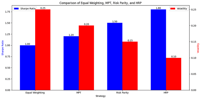
This approach goes beyond individual asset risks, recognizing the complex web of correlations that truly influence a portfolio’s performance. Moreover, as depicted below, given the same set of assets, one would expect a higher Sharpe Ratio and lower volatility by implementing HRP.


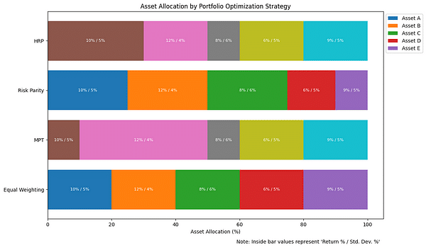
Figure 1. This visual representation contrasts asset allocation decisions with their associated Sharpe Ratios and volatilities. Asset allocations showcase how each method diversifies investments among various assets to achieve its risk-return objectives. The Sharpe Ratios elucidate risk-adjusted returns, measuring the return earned per unit of risk. Volatilities illustrate the inherent risk levels of each strategy.
2. Understanding Hierarchical Clustering in HRP
2.1 Tree Structures and Dendrogram
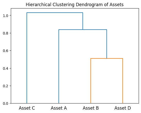
Hierarchical clustering groups data over a series of steps, creating a tree of clusters called a dendrogram.
Furthermore, this method does not pre-assume any number of clusters, which can be determined by cutting the dendrogram at a level.


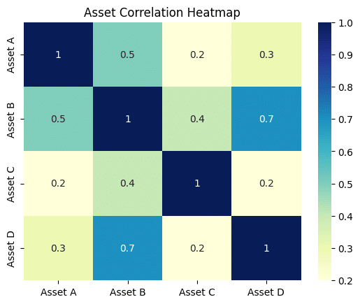
Figure 2. Visualizing Asset Relationships in HRP. The dendrogram (top) illustrates the hierarchical clustering of assets, showcasing the multi-level tree structure used to group assets based on similarity. A correlation heatmap (bottom) provides a color-coded representation of the pairwise correlations between assets, serving as the foundation for constructing the dendrogram in the HRP process.
Dendograms visually demonstrate the clustering of assets based on their similarities. For a visual representation of the asset allocation derived from hierarchical clustering, you can use a heatmap. This heatmap can depict the correlation between assets, with warmer colors indicating a higher correlation.
2.2 Basics of Hierarchical Clustering
Hierarchical clustering takes place in two approaches:
- Agglomerative (bottom-up): It starts with each observation as a separate cluster and merges them based on similarity.
- Divisive (top-down): It starts with all observations in one cluster and divides them.
Mathematically, the similarity between two clusters can be represented using various metrics, but in the context of HRP, the distance d between two clusters X and Y can be given by:

Equation 4. This equation defines the Euclidean distance d(X,Y) between two data points X and Y in an n-dimensional space, which is commonly used in the agglomerative approach of hierarchical clustering within HRP.
Where xi and yi are individual data points in clusters X and Y respectively.
2.3 From Clusters to Asset Allocation
Once we’ve identified the asset clusters, the next step is understanding how to allocate investments among these clusters and within clusters.
Furthermore, with Hierarchical Risk Parity, the process goes beyond just the hierarchical clustering. Allocation also depends on the inverse-variance weights of the clusters. This is derived from the hierarchy structure and the covariance matrix of the assets.
Allocation of w to a particular cluster or asset is inversely proportional to its variance σ2:

Equation 5. Inverse-Variance Weighting in HRP: In this allocation strategy, the weight w assigned to an asset or cluster is inversely proportional to its variance σ2. It ensures that assets with higher risk (higher variance) are assigned a lower weight, promoting a risk-adjusted investment approach within the hierarchical framework.
This method ensures that assets or clusters with higher uncertainty receive a lower weight in the portfolio, thereby leading to a more robust portfolio allocation.
2.4 Relevance of tree structures in finance
In finance, assets that move together under various market scenarios can be treated as a group. Hierarchical clustering provides a systematic way to identify these groups.
Moreover, by understanding the nested hierarchy of assets, a portfolio manager can diversify assets at multiple levels: within clusters and between clusters.
3. Constructing an HRP Portfolio
Hierarchical Risk Parity considers both the individual variances of assets and their pairwise covariances.
In contrast, unlike other methodologies that can be dominated by a few highly volatile assets, HRP ensures diversification by grouping correlated assets together.
3.1 Covariance Matrix and Correlation Matrix
At the heart of portfolio construction is the correlation matrix, a table showing correlation coefficients between variables.
Furthermore, the correlation matrix is derived from the covariance matrix, and both are instrumental in understanding the relationships between assets.
Lastly, the covariance provides a measure of the joint variability of two random variables. In the correlation matrix, these values are standardized to fall between -1 and 1, making them interpretable as a linear relationship.
					# Calculating the covariance and correlation matrices
covariance_matrix = Y.cov()
correlation_matrix = Y.corr()
3.2 Clustering
Grouping assets based on their correlation allows for a hierarchical view, which aids in optimizing asset allocations. It identifies clusters of assets that behave similarly.
Agglomerative Clustering
Agglomerative clustering is a bottom-up hierarchical clustering method. Initially, it treats each object as a singleton cluster and then progressively merges clusters until all clusters have been merged into one big cluster containing all objects.
Moreover, Riskfolio-Lib, a Python library, offers functionalities to visualize these clusters using a dendrogram:
					# Plotting the dendrogram for asset clusters
ax = rp.plot_dendrogram(returns=Y,
                        codependence='pearson',
                        linkage='single',
                        k=None,
                        max_k=10,
                        leaf_order=True,
                        ax=None)
Minimum Spanning Tree (MST)
MST connects all assets in a way where the total weight or distance between them is minimized, ensuring there aren’t any cycles. In the context of portfolio optimization, MST ensures that only the most essential relationships (edges) between assets are maintained.
Need comprehensive financial data to make better analyses and investment decisions? Get it with Financial Modeling Prep. Click for a 15% discount with Entreprenerdly.
3.3 Complete Python Implementation
Combining all the pieces together gives us a comprehensive code to construct an HRP portfolio.
The given Python code first fetches data for a list of assets, calculates their returns, visualizes the hierarchical clusters, and finally uses Riskfolio-Lib to generate the optimal HRP portfolio.
Taking S&P500 companies as a model, we discerned how HRP comprehends both individual asset characteristics and their correlations. As markets persist in evolving, harnessing methods like HRP can be invaluable.
Related Article
Optimize Portfolio Performance with Risk Parity Rebalancing in Python

Newsletter
