Optimal ATR Multiples by Clustering EMA-Based Performance Metrics for Deriving Buy and Sell Signals with
What if your trend indicator could tune itself with no optimization, no backtesting, or no overfitting?
That’s the idea behind the indicator presented in this analysis. Instead of manually choosing parameters, we built a SuperTrend variant that adapts its sensitivity based on how price behaves.
It uses its own performance as feedback, clusters the results, and selects the best configuration in real time.
No predictive modeling. No supervised learning. Just price action, a custom scoring function, and unsupervised clustering.
This article walks through the entire architecture — from parameter sweeping and performance metrics to k-means clustering and final signal reconstruction.
This article is structured as follows:
- The Self-Tuning Trend System
- Python Implementation
- Applications and Extentions
End-to-end Python Notebook provided below.
1. A Self-Tuning Trend Signal
Most technical indicators rely on fixed parameters. You pick a multiplier, a moving average length, or a threshold and hope it works across time.
But markets don’t stay constant. Volatility shifts. Trends evolve. What worked last month breaks down the next.
The SuperTrend flips bullish when price closes above a dynamic upper band and flips bearish when it closes below a lower band — those flips are your buy and sell signals.
Instead of picking a single setting, we let the system explore a range of ‘SuperTrend’ configurations. Then we score each one based on how well it tracked the price.
Here’s the core idea:
1. Build multiple SuperTrend signals using different multipliers:
Instead of using one multiplier (say, 3.0), we test a range — from 1.0 to 5.0 in small steps. Each version creates a different set of signals.
The SuperTrend levels are calculated using the formula:
2. Score each version using a custom, price-based performance metric.
We look at each version and track whether the price moves in the expected direction after the signal flips.
We measure this using a custom performance metric. It works like a memory:
- If the signal flips and the price moves in that direction, the score goes up.
- If the signal flips and price moves the other way, it drops.
The scoring system uses this smoothed formula:

This rewards signals that actually lead price in the right direction.
3. Cluster the results using unsupervised learning (k-means, k=3). This groups all tested multipliers into:
- Best-performing signals
- Average signals
- Poor-performing signals
So instead of picking the highest score directly, we let k-means do the job.
4. Rebuild the indicator using the “Best” group.
Once we know which group performed best, we take the average multiplier from that group, maybe it’s 2.5, maybe it’s 4.2, and use it to compute a final SuperTrend.
Implementation architecture can be summarized with the following diagram:
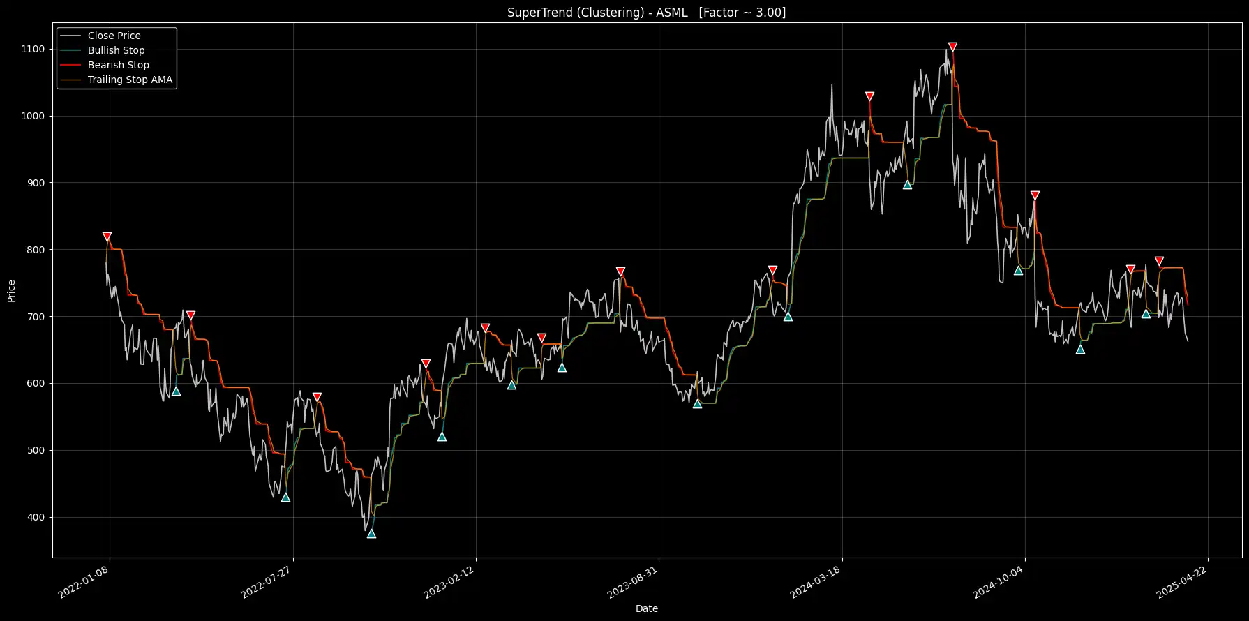
Figure 1. Architecture Diagram: Trading Signals with Adaptive SuperTrend and K-Means Clustering
2. Python Implementation
2.1 Define Core Inputs and Signal Settings
The ticker, start date, and end date control which asset is analyzed and over what time period. You can apply the system to any stock, ETF, or crypto pair by changing the ticker.
ATR length determines how volatility is measured. A lower value makes the ATR more sensitive to recent price spikes, leading to faster but potentially noisier signals. A higher value smooths the ATR and reduces false flips, but may delay trend detection.
The SuperTrend multipliers define the range of sensitivity the system will test — from tighter stops (lower values) to wider ones (higher values). The STEP
size controls how granular that testing is. A finer step gives more choices but takes longer to compute.
PERF_ALPHA affects how the system scores each SuperTrend version. Lower values make the performance metric more responsive to recent changes. Higher values favor long-term stability.
FROM_CLUSTER tells the model which group of signals to trust — Best, Average, or Worst. Most users will select “Best” for trend-following strategies.
Finally, MAX_ITER caps how long the k-means clustering runs. Higher values allow more precise grouping but increase computation time.
import numpy as np
import pandas as pd
import matplotlib.pyplot as plt
import matplotlib.dates as mdates
import matplotlib.style as mplstyle
import yfinance as yf
# User parameters
TICKER = "ASML" # Ticker symbol to pull from Yahoo Finance
# Time range for the analysis
START_DATE = "2022-01-01"
END_DATE = "2025-12-01"
# ATR_LENGTH controls how reactive the ATR (Average True Range) is.
# Shorter = more sensitive to price spikes. Longer = smoother.
ATR_LENGTH = 10
# These define the range of SuperTrend factors to test.
# We'll run the SuperTrend indicator across multiple values between MIN_MULT and MAX_MULT.
MIN_MULT = 1.0 # smallest factor (tightest stop)
MAX_MULT = 5.0 # largest factor (widest stop)
STEP = 0.5 # spacing between factors (e.g., 1.0, 1.5, 2.0, ...)
# PERF_ALPHA controls smoothing of the performance metric.
# Lower = more reactive to recent price behavior.
PERF_ALPHA = 10
# We'll cluster the performance results into 3 groups (Best, Average, Worst)
# and select the factor from the chosen group.
FROM_CLUSTER = "Best" # Options: "Best", "Average", or "Worst"
# Maximum number of iterations for the k-means clustering step
MAX_ITER = 1000
# Note: maxData isn't needed here, but could be used to limit data length if desired.
2.2 Fetch and Prepare Market Data
Historical price data for the chosen ticker (e.g, ASML) is downloaded from Yahoo Finance.
Key columns (High, Low, Close) are retained, and the mid-price is computed as:
# 1) Download data
df = yf.download(TICKER, start=START_DATE, end=END_DATE, interval="1d", auto_adjust=False)
if df.empty:
raise ValueError("No data returned from yfinance")
# Flatten multi-index columns if needed
if isinstance(df.columns, pd.MultiIndex):
df.columns = df.columns.get_level_values(0)
# For safety, rename columns so we can do df["High"], etc.
df.rename(columns={"Open":"Open", "High":"High", "Low":"Low", "Close":"Close", "Volume":"Volume"}, inplace=True)
df.dropna(subset=["High","Low","Close"], inplace=True)
# hl2
df["hl2"] = (df["High"] + df["Low"]) / 2.0
2.3 Measure Volatility with ATR
We use a 10-bar Average True Range to measure volatility. It can capture both intraday movement and overnight gaps.
First, we compute the True Range, TR, for each bar:
Then we smooth it using an Exponential Moving Average EMA:
This dynamic measure expands in volatile markets and contracts in stable ones. It becomes the foundation for the SuperTrend bands that follow.
Newsletter