The Fundamentals, Adaptive and Dynamic, Advanced Weighting and From Niche to Noteworthy
Moving averages are one of the most widely used technical indicators by traders and investors of all levels. They help to smooth out the inherent volatility of stock prices by calculating the average price over a specified period. Moving averages can be simple to calculate, but there are also more complex forms that are designed to capture more nuance aspects of the market.
This article will discuss a total of 36 different moving average methods, from the foundational to the more sophisticated and niche. We will cover the methodology and implementation of each method, and provide the Python code for you to plug and play.
Methods are grouped as follows:
- Fundamental Techniques: Simple Moving Average (SMA), Exponential Moving Average (EMA), Weighted Moving Average (WMA), Double Exponential Moving Average (DEMA), Triple Exponential Moving Average (TEMA), Volume Adjusted Moving Average (VAMA), Adaptive Moving Average (AMA or KAMA), Triangular Moving Average (TMA), Hull Moving Average (HMA)
- Adaptive and Dynamic: Fractal Adaptive Moving Average (FRAMA), Zero Lag Exponential Moving Average (ZLEMA), Variable Index Dynamic Average (VIDYA), Arnaud Legoux Moving Average (ALMA), MESA Adaptive Moving Average (MAMA), Following Adaptive Moving Average (FAMA) , Adaptive Period Moving Average, Rainbow Moving Average, Wilders Moving Average, Smoothed Moving Average (SMMA)
- Advanced Weighting: Guppy Multiple Moving Average (GMMA), Least Squares Moving Average (LSMA), Welch’s Moving Average or Modified Moving Average, Sin-weighted Moving Average, Median Moving Average, Geometric Moving Average, Elastic Volume Weighted Moving Average (eVWMA), Regularized Exponential Moving Average (REMA), Parabolic Weighted Moving Average
- From Niche to Noteworthy: Jurik Moving Average (JMA), End Point Moving Average (EPMA), Chande Moving Average (CMA), Harmonic Moving Average, McGinley Dynamic, Anchored Moving Average, Holt-Winters Moving Average, Filtered Moving Average, Kijun Sen (Base Line
2. Fundamental Techniques
This section explores the methodologies from both theoretical and practical standpoints. The ultimate goal is to offer a Python-based implementation to put them all to work.
2.1 Simple Moving Average (SMA)
The Simple Moving Average, commonly referred to as SMA, is one of the most basic and commonly used technical analysis tools. At its core, the SMA calculates the average price of a security over a set number of periods.
This average smoothens out short-term price fluctuations, allowing traders to understand the underlying trend of the stock. The longer the period chosen for the SMA, the smoother the curve; however, it might also lag behind the actual price movements.
Mathematical Representation of the Simple Moving Average (SMA) for a Defined Period.
When a stock price exceeds its SMA, it’s typically seen as a bullish sign, indicating potential upward movement. Conversely, falling below the SMA suggests a possible downtrend.
The “crossover” strategy is also prevalent, where traders observe a short and long-term SMA. A bullish sign is noted when the short-term crosses above the long-term, and vice versa for a bearish signal.
					# Required Libraries
import yfinance as yf
import matplotlib.pyplot as plt
import pandas as pd

# Fetch data
ticker_symbol = "AAPL"
data = yf.download(ticker_symbol, start="2020-01-01", end="2024-01-01")

# Calculate SMA
sma_period = 50  # Example: 50 days SMA
data['SMA'] = data['Close'].rolling(window=sma_period).mean()

# Plot
plt.figure(figsize=(20,7))
plt.plot(data['Close'], label=f'{ticker_symbol} Stock Price', color='blue')
plt.plot(data['SMA'], label=f'{sma_period} Day SMA', color='red', linestyle='--')
plt.title(f'{ticker_symbol} Stock Price with 50 Day SMA (n={sma_period})')
plt.xlabel('Date')
plt.ylabel('Stock Price')
plt.legend()
plt.grid(True)
plt.tight_layout()
plt.show()
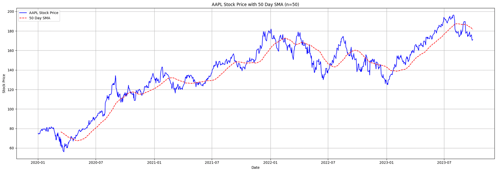
Figure. 1: Apple Inc. (AAPL) Stock Price and its 50-Day Simple Moving Average (SMA) from 2020 to 2023.
2.2 Exponential Moving Average (EMA)
The Exponential Moving Average (EMA) is another vital tool in technical analysis, but unlike the SMA, it gives more weight to the most recent prices. This weighting provides the EMA with a slight advantage over the SMA, as it reacts more quickly to price changes.
The primary benefit of the EMA is its sensitivity, making it a preferred choice when determining short-term price movements and potential market entry and exit points.
Formula for the Exponential Moving Average (EMA) with Smoothing Factor α.
- EMAt is the Exponential Moving Average for the current time t
- Pt is the price for the current time t
- α is the smoothing factor, calculated as α = 2 / (N+1)
- N is the period of the EMA
- EMAt−1 is the Exponential Moving Average for the previous time t−1
The EMA’s rapid reaction to price fluctuations is both its strength and challenge. Its heightened sensitivity provides quick insights, making it invaluable for tracking short-term market movements.
However, this very trait can sometimes amplify the effects of short-term volatility, potentially leading to reactive or mistimed trades.
					# Required Libraries
import yfinance as yf
import matplotlib.pyplot as plt
import pandas as pd

# Fetch data
ticker_symbol = "MSFT"
data = yf.download(ticker_symbol, start="2020-01-01", end="2024-01-01")

# Calculate EMA
ema_period = 50
data['EMA'] = data['Close'].ewm(span=ema_period, adjust=False).mean()

# Plot
plt.figure(figsize=(20,7))
plt.plot(data['Close'], label=f'{ticker_symbol} Stock Price', color='blue')
plt.plot(data['EMA'], label=f'50 Day EMA', color='green', linestyle='--')
plt.title(f'{ticker_symbol} Stock Price with 50 Day EMA')
plt.xlabel('Date')
plt.ylabel('Stock Price')
plt.legend()
plt.grid(True)
plt.tight_layout()
plt.show()
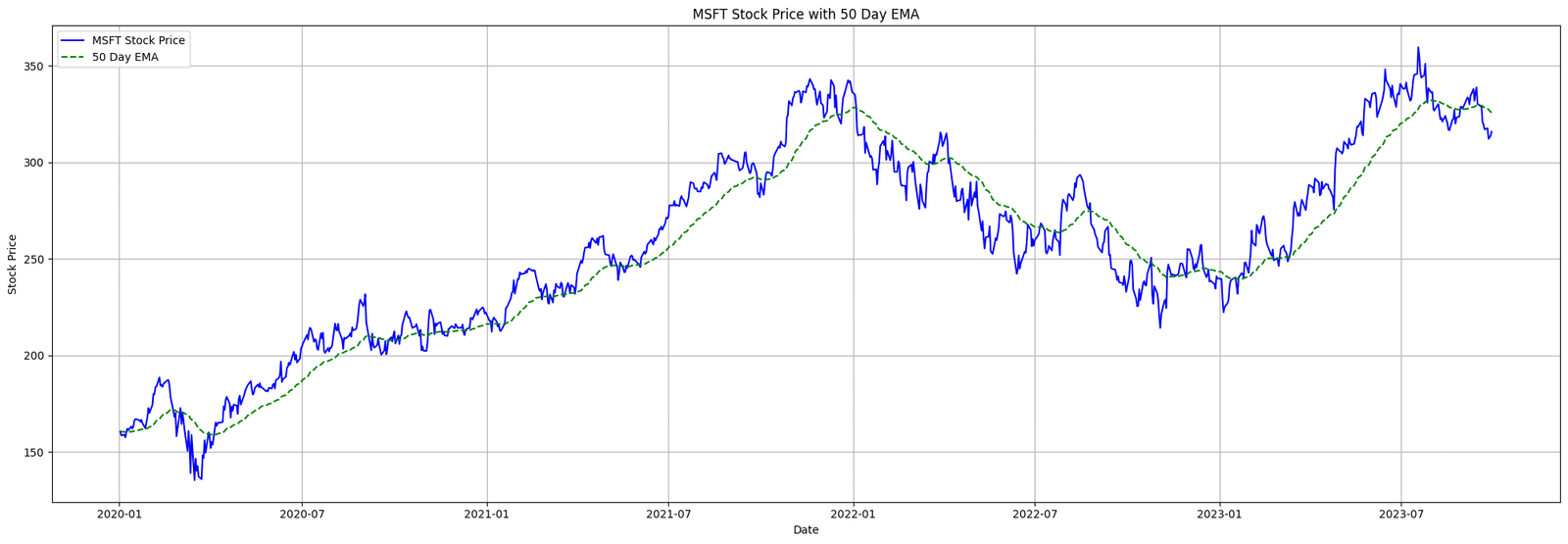
Figure. 2: Microsoft Corporation (MSFT) Stock Price and its 50-Day Exponential Moving Average (EMA) from 2020 to 2023.
2.3 Weighted Moving Average (WMA)
The Weighted Moving Average (WMA) assigns a weight to each data point based on its age. Unlike the SMA which gives equal weight to all data points, the WMA gives more importance to the recent prices, and less importance to older prices.
Essentially, this method allows traders to highlight recent movements in prices over older ones, capturing potential trends earlier than the SMA. The WMA is commonly used for short-term price forecasting.
The WMA is calculated using the following formula:

Equation. 3: Mathematical Expression for the Weighted Moving Average (WMA) with Defined Weights.
- Pi is the price for the ith period.
- wi is the weight assigned to the price for the ith period.
- N is the period of the WMA.
Application
Typically, weights decrease linearly. For example, for a 3-day WMA, the most recent day’s price might be multiplied by 3, the previous day by 2, and the oldest day by 1.
The nuanced weighting mechanism of the WMA provides a distinctive edge in capturing emerging market trends. Its design inherently leans into recent market activities.
However, this very emphasis on recent data means the WMA might be more susceptible to short-term market noise or volatility. For traders who prioritize recent market actions, the WMA can be a potent asset.
					# Required Libraries
import yfinance as yf
import matplotlib.pyplot as plt
import pandas as pd
import numpy as np

# Fetch data
ticker_symbol = "META"
data = yf.download(ticker_symbol, start="2020-01-01", end="2024-01-01")

# Calculate WMA
wma_period = 50  # Example: 50 days WMA
weights = np.arange(1, wma_period + 1)
data['WMA'] = data['Close'].rolling(window=wma_period).apply(lambda prices: np.dot(prices, weights)/weights.sum(), raw=True)

# Plot
plt.figure(figsize=(20,7))
plt.plot(data['Close'], label=f'{ticker_symbol} Stock Price', color='blue')
plt.plot(data['WMA'], label=f'{wma_period} Day WMA', color='orange', linestyle='--')
plt.title(f'{ticker_symbol} Stock Price with {wma_period} Day WMA')
plt.xlabel('Date')
plt.ylabel('Stock Price')
plt.legend()
plt.grid(True)
plt.tight_layout()
plt.show()
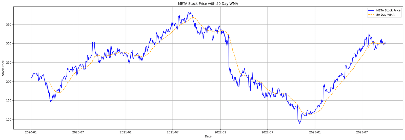
Figure. 3: Meta Platforms, Inc. (META) Stock Price with its 50-Day Weighted Moving Average (WMA) from 2020 to 2023, showcasing the dynamic weighting emphasis on recent prices.
2.4 Double Exponential Moving Average (DEMA)
The Double Exponential Moving Average (DEMA) is a refinement of the traditional EMA, designed to be more responsive to recent price changes. It’s an attempt to reduce the lag inherent in simple moving averages or even EMAs.
The DEMA does this by taking the difference between a single EMA and a double EMA and adding it back to the original EMA. Because of this, DEMA reacts more quickly to price changes than the traditional EMA.
1. Calculate the EMA over period N
Exponential Moving Average (EMA) for a period of N day.
2. Calculate the EMA of EMA_N over the same period
Exponential Moving Average of the first EMA, both spanning N days.
3. The DEMA is given by:
Formulation of the Double Exponential Moving Average (DEMA) for Enhanced Trend Sensitivity.
Where:
- P is the price for the current period.
- α is the smoothing constant, and it’s equal to 2 / (N+1)
The DEMA’s heightened responsiveness makes it particularly appealing for traders who wish to act on swift market changes. When prices exhibit rapid fluctuations, the DEMA is more adept at highlighting emerging trends or reversals, potentially offering a trader an advantageous entry or exit point. This becomes especially valuable in volatile markets where timeliness can make a significant difference.
					# Required Libraries
import yfinance as yf
import matplotlib.pyplot as plt
import pandas as pd

# Fetch data
ticker_symbol = "ASML"
data = yf.download(ticker_symbol, start="2020-01-01", end="2024-01-01")

# Calculate DEMA
dema_period = 50
alpha = 2 / (dema_period + 1)
data['EMA'] = data['Close'].ewm(span=dema_period, adjust=False).mean()
data['EMA2'] = data['EMA'].ewm(span=dema_period, adjust=False).mean()
data['DEMA'] = 2 * data['EMA'] - data['EMA2']

# Plot
plt.figure(figsize=(20,7))
plt.plot(data['Close'], label=f'{ticker_symbol} Stock Price', color='blue')
plt.plot(data['DEMA'], label=f'{dema_period} Day DEMA', color='red', linestyle='--')
plt.title(f'{ticker_symbol} Stock Price with {dema_period} Day DEMA')
plt.xlabel('Date')
plt.ylabel('Stock Price')
plt.legend()
plt.grid(True)
plt.tight_layout()
plt.show()
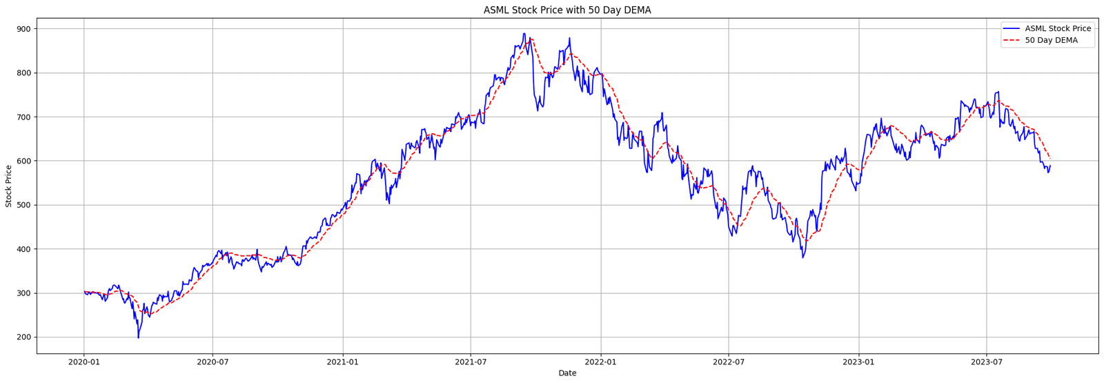
Figure. 4: ASML Holding N.V. (ASML) Stock Price plotted against its 50-Day Double Exponential Moving Average (DEMA) from 2020 to 2023, illustrating DEMA’s enhanced responsiveness to price changes.
2.5 Triple Exponential Moving Average (TEMA)
The Double Exponential Moving Average (DEMA) is a refinement of the traditional EMA, designed to be more responsive to recent price changes. It’s an attempt to reduce the lag inherent in simple moving averages or even EMAs.
The DEMA does this by taking the difference between a single EMA and a double EMA and adding it back to the original EMA. Because of this, DEMA reacts more quickly to price changes than the traditional EMA.
The Triple Exponential Moving Average (TEMA) is another enhancement of the EMA. It aims to further reduce the lag and noise associated with single and double EMAs.
TEMA essentially triples the weighting of recent prices to become even more sensitive to price changes. It’s calculated using three EMAs: a single EMA, a double EMA (DEMA), and a triple EMA. By subtracting out the “lagged” effects of the first two, TEMA becomes highly responsive.
1.Calculate the EMA over period N
Exponential Moving Average (EMA) for a period of N days.
2. Calculate the EMA of EMA_N over the same period
Secondary Exponential Moving Average calculated from the EMA of period N days.
3. Calculate the EMA of EMA_N,2 over the same period
Tertiary Exponential Moving Average derived from the second EMA of period N days.
4. The TEMA is then given by:
Triple Exponential Moving Average (TEMA) combining the three EMAs.
Where:
- P is the price for the current period.
- α is the smoothing constant, and it’s equal to 2/(N+1)
By tripling down on recent price movements, TEMA stands out as a tool finely tuned to the market’s immediate dynamics. This makes it invaluable in volatile trading conditions where capturing subtle shifts is crucial. Yet, its sharp sensitivity can also elevate the risk of overvaluing fleeting price deviations. As a result, traders using TEMA must exercise discernment to distinguish authentic market movements from transient anomalies.
					# Required Libraries
import yfinance as yf
import matplotlib.pyplot as plt
import pandas as pd

# Fetch data
ticker_symbol = "TSLA"
data = yf.download(ticker_symbol, start="2020-01-01", end="2024-01-01")

# Calculate TEMA
tema_period = 50
alpha = 2 / (tema_period + 1)
data['EMA'] = data['Close'].ewm(span=tema_period, adjust=False).mean()
data['EMA2'] = data['EMA'].ewm(span=tema_period, adjust=False).mean()
data['EMA3'] = data['EMA2'].ewm(span=tema_period, adjust=False).mean()
data['TEMA'] = 3 * data['EMA'] - 3 * data['EMA2'] + data['EMA3']

# Plot
plt.figure(figsize=(20,7))
plt.plot(data['Close'], label=f'{ticker_symbol} Stock Price', color='blue')
plt.plot(data['TEMA'], label=f'{tema_period} Day TEMA', color='green', linestyle='--')
plt.title(f'{ticker_symbol} Stock Price with {tema_period} Day TEMA')
plt.xlabel('Date')
plt.ylabel('Stock Price')
plt.legend()
plt.grid(True)
plt.tight_layout()
plt.show()
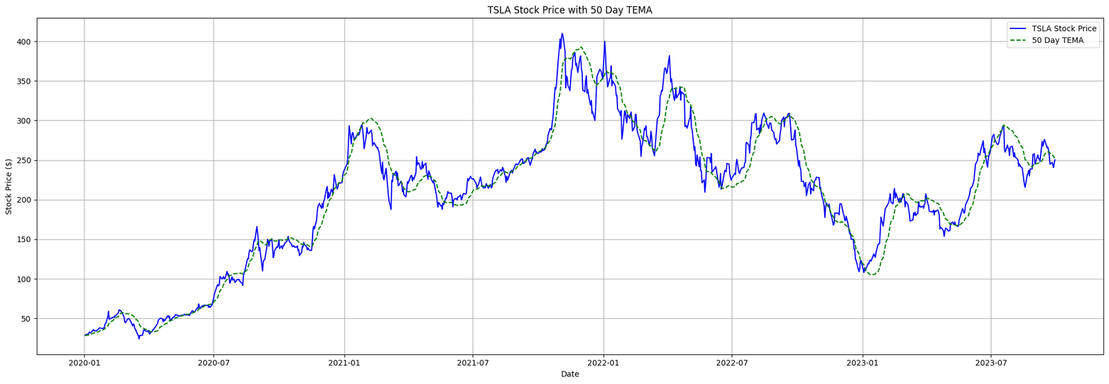
Figure. 5: Tesla, Inc. (TSLA) Stock Price with its 50-Day Triple Exponential Moving Average (TEMA) from 2020 to 2023, showcasing TEMA’s advanced filtering of price noise.
2.6 Volume Adjusted Moving Average (VAMA)
The Volume Adjusted Moving Average (VAMA) integrates volume data into the moving averages calculation, thereby giving more importance to prices that are accompanied by higher volume.
This means that during periods of higher trading activity, the VAMA will give more weight to the current price, making it more responsive. VAMA can be especially useful in identifying the strength of price movements, as large moves backed by substantial volume might be more sustainable.

Volume Adjusted Moving Average (VAMA) accounting for the significance of volume in price movements over a specified period N.
Where:
- Pi is the closing price for period i.
- Vi is the trading volume for period i.
- N is the specified number of periods.
Application
When a significant price change is backed by high volume, it often signals a stronger consensus among traders about the asset’s value, making VAMA particularly adept at highlighting robust trends.
One of the main criticisms of VAMA is that it may not respond as quickly to changes in price and volume. Since EVWMA addresses this shortcoming by placing a larger weight on recent data (both in terms of price and volume), therefore, being more reactive to recent market events. EVWMA is further discussed in article 3 of this series.
					# Required Libraries
import yfinance as yf
import matplotlib.pyplot as plt
import pandas as pd

# Fetch data
ticker_symbol = "NVDA"
data = yf.download(ticker_symbol, start="2020-01-01", end="2024-01-01")

# Calculate VAMA
vama_period = 50
data['Volume_Price'] = data['Close'] * data['Volume']
data['VAMA'] = data['Volume_Price'].rolling(window=vama_period).sum() / data['Volume'].rolling(window=vama_period).sum()

# Plot
plt.figure(figsize=(20,7))
plt.plot(data['Close'], label=f'{ticker_symbol} Stock Price', color='blue')
plt.plot(data['VAMA'], label=f'{vama_period} Day VAMA', color='orange', linestyle='--')
plt.title(f'{ticker_symbol} Stock Price with {vama_period} Day VAMA')
plt.xlabel('Date')
plt.ylabel('Stock Price')
plt.legend()
plt.grid(True)
plt.tight_layout()
plt.show()
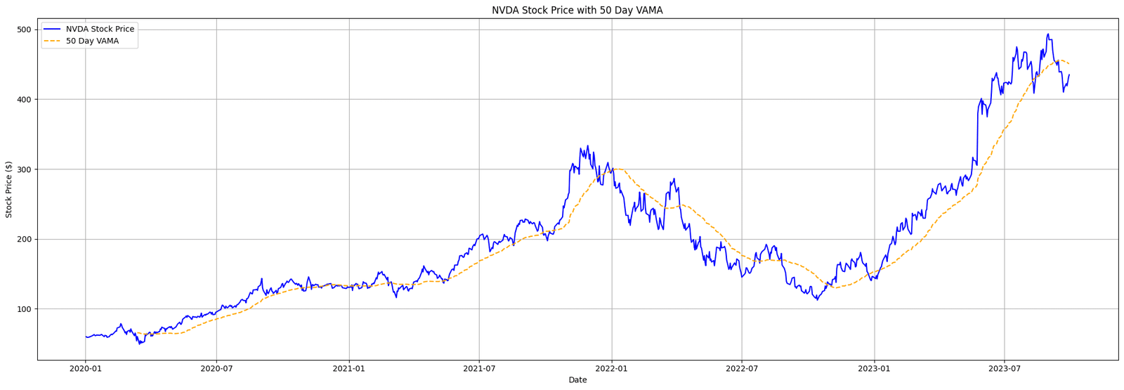
Figure. 6: NVIDIA Corporation (NVDA) Stock Price compared with its 50-Day Volume-Adjusted Moving Average (VAMA) from 2020 to 2023, emphasizing the influence of trading volume on price movement.
2.7 Adaptive Moving Average (AMA or KAMA)
KAMA was developed by Perry Kaufman and is designed to be more responsive to price changes compared to other moving averages. The key feature of KAMA is its adaptability: it adjusts the smoothing constant based on the market’s volatility.
When the price moves in a strong trend, KAMA becomes more sensitive, and during range-bound, sideways market conditions, KAMA becomes smoother to filter out noise.
This adaptability is achieved through the Efficiency Ratio (ER), which measures the price directionality and volatility, and the Smoothing Constant (SC), which is derived from the ER and defines the weight given to the most recent price data.

Efficiency Ratio (ER) representing the price change rate relative to its volatility.
Determination of the Smoothing Constant (SC) using the Efficiency Ratio, fastest SC, and slowest SC.
Calculation of Kaufman’s Adaptive Moving Average (KAMA) by incorporating the dynamic Smoothing Constant.
Where:
- ER is the Efficiency Ratio.
- SC is the Smoothing Constant.
- The fastest SC and the slowest SC are typically set at 2/(2+1) and 2/(30+1) respectively.
Application
By dynamically adjusting its sensitivity based on market volatility, KAMA offers traders a unique blend of responsiveness and stability. During times of pronounced price trends, KAMA intensifies its sensitivity, enabling traders to pinpoint potential breakout or breakdown scenarios.
On the other hand, in more subdued, lateral market phases, KAMA showcases its versatility by tempering responses to trivial price shifts, thereby lessening the likelihood of misleading indicators.
					# Required Libraries
import yfinance as yf
import matplotlib.pyplot as plt
import pandas as pd

# Fetch data
ticker_symbol = "BRK-B"
data = yf.download(ticker_symbol, start="2020-01-01", end="2024-01-01")

# Calculate KAMA
n = 10
fastest_SC = 2 / (2 + 1)
slowest_SC = 2 / (30 + 1)

data['Change'] = abs(data['Close'] - data['Close'].shift(n))
data['Volatility'] = data['Close'].diff().abs().rolling(window=n).sum()

data['ER'] = data['Change'] / data['Volatility']
data['SC'] = (data['ER'] * (fastest_SC - slowest_SC) + slowest_SC)**2

data['KAMA'] = data['Close'].copy()
for i in range(n, len(data)):
    data['KAMA'].iloc[i] = data['KAMA'].iloc[i-1] + data['SC'].iloc[i] * (data['Close'].iloc[i] - data['KAMA'].iloc[i-1])

# Plot
plt.figure(figsize=(20,7))
plt.plot(data['Close'], label=f'{ticker_symbol} Stock Price', color='blue')
plt.plot(data['KAMA'], label=f'KAMA (n={n})', color='green', linestyle='--')
plt.title(f'{ticker_symbol} Stock Price with KAMA (n={n})')
plt.xlabel('Date')
plt.ylabel('Stock Price')
plt.legend()
plt.grid(True)
plt.tight_layout()
plt.show()

Figure. 7: Berkshire Hathaway Inc. Class B (BRK-B) Stock Price with its Kaufman’s Adaptive Moving Average (KAMA) from 2020 to 2023, illustrating the adaptive nature of KAMA based on price volatility.
2.8 Triangular Moving Average (TMA)
The Triangular Moving Average is a type of smoothed moving average that puts the most weight on the middle prices of the dataset. It’s essentially an average of an average, providing a smoothing effect that’s more profound than the Simple Moving Average.
Due to the added smoothing, the TMA can lag behind price more than other moving averages, but this can be advantageous when trying to eliminate insignificant price fluctuations.

Calculation of the Triangular Moving Average (TMA) emphasizing the central prices by using a weighted Simple Moving Average (SMA).
- SMA(t, n+1/2 ) is the SMA at time t over n+1/2 periods.
- t is the current period.
- n is the number of periods chosen for the TMA.
Application
The Triangular Moving Average offers traders a uniquely smoothed perspective on price trends. Its double-layered averaging process filters out the short-term market noise more efficiently than the Simple Moving Average.
This deliberate lag is TMA’s strength when traders aim to sidestep inconsequential price movements and focus on overarching trends. However, the very quality that makes TMA a formidable noise reducer can also cause it to react slower to genuine market shifts.
					# Required Libraries
import yfinance as yf
import matplotlib.pyplot as plt
import pandas as pd

# Fetch data
ticker_symbol = "GOOGL"
data = yf.download(ticker_symbol, start="2020-01-01", end="2024-01-01")

# Calculate TMA
n = 20
half_n = (n+1) // 2
data['Half_SMA'] = data['Close'].rolling(window=half_n).mean()
data['TMA'] = data['Half_SMA'].rolling(window=half_n).mean()

# Plot
plt.figure(figsize=(20,7))
plt.plot(data['Close'], label=f'{ticker_symbol} Stock Price', color='blue')
plt.plot(data['TMA'], label=f'TMA (n={n})', color='red', linestyle='--')
plt.title(f'{ticker_symbol} Stock Price with TMA (n={n})')
plt.xlabel('Date')
plt.ylabel('Stock Price')
plt.legend()
plt.grid(True)
plt.tight_layout()
plt.show()
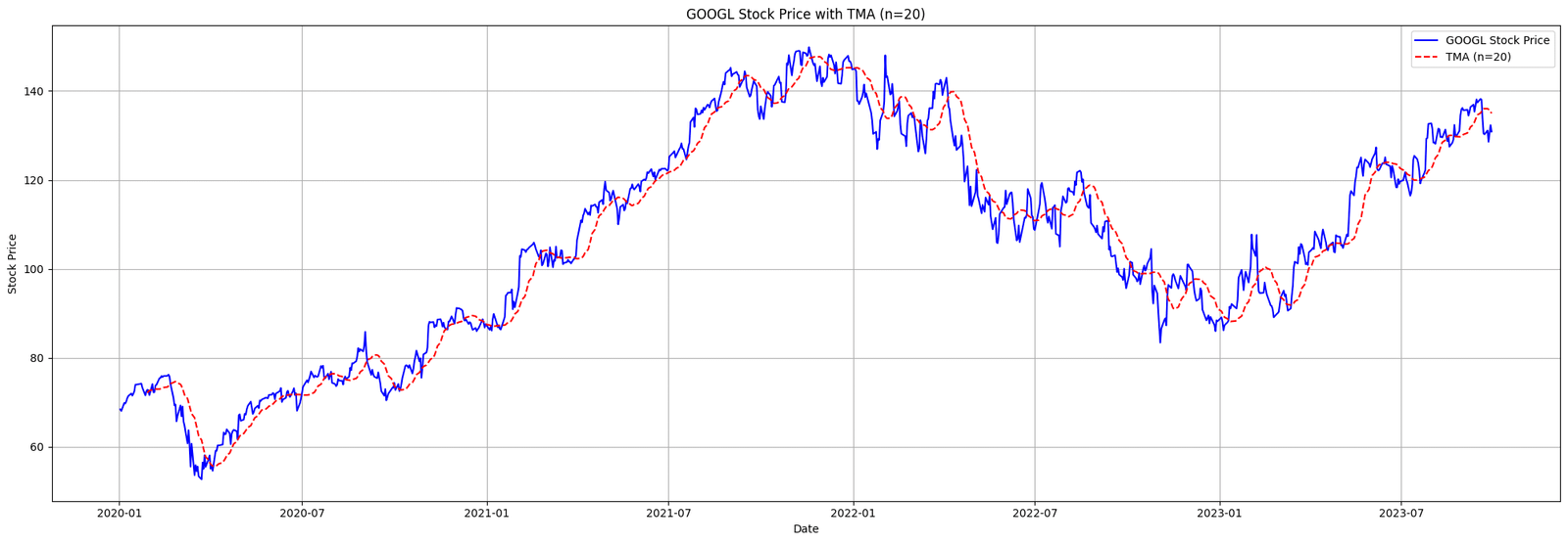
Figure. 8: Alphabet Inc. (GOOGL) Stock Price alongside its Triangular Moving Average (TMA) from 2020 to 2023, showcasing the profound smoothing effect of the TMA on the stock’s price movements.
2.9 Hull Moving Average (HMA)
The Hull Moving Average is designed to eliminate lag and improve smoothing, making it responsive to current prices. Alan Hull developed this average to keep up with price action while maintaining a curve that’s smooth.
By taking the weighted average of the SMA, and then further smoothing it, HMA minimizes the lag of traditional moving averages while emphasizing recent prices. Below are the steps to calculate HMA:
- Calculate a Weighted Moving Average with period n / 2 (which is just half of the period you want to use).
- Calculate a Weighted Moving Average for period n.
- Calculate the sqrt(n) weighted moving average of the difference between the two averages (from step 1 and 2).
Steps and formulas for calculating the Hull Moving Average (HMA), designed to provide a responsive yet smooth representation of price action.
Where:
- WMA(n) is the weighted moving average over n periods.
- t is the current period.
- n is the number of periods chosen for the HMA.
Application
By fusing responsiveness with smoothness, the Hull Moving Average presents traders with a tool adept at capturing contemporary price dynamics without the clutter of short-lived fluctuations. Alan Hull’s design prioritizes recent prices, yet by doubly smoothing the average, the HMA ensures that its curve isn’t jolted by every market hiccup.
					# Required Libraries
import yfinance as yf
import matplotlib.pyplot as plt
import numpy as np

def weighted_moving_average(data, periods):
    weights = np.arange(1, periods + 1)
    wma = data.rolling(periods).apply(lambda x: np.dot(x, weights) / weights.sum(), raw=True)
    return wma

def hull_moving_average(data, periods):
    wma_half_period = weighted_moving_average(data, int(periods / 2))
    wma_full_period = weighted_moving_average(data, periods)
    hma = weighted_moving_average(2 * wma_half_period - wma_full_period, int(np.sqrt(periods)))
    return hma

# Fetch data
ticker_symbol = "JPM"
data = yf.download(ticker_symbol, start="2020-01-01", end="2024-01-01")

# Calculate HMA
n = 120
data['HMA'] = hull_moving_average(data['Close'], n)

# Plot
plt.figure(figsize=(20,7))
plt.plot(data['Close'], label=f'{ticker_symbol} Stock Price', color='blue')
plt.plot(data['HMA'], label=f'HMA (n={n})', color='green', linestyle='--')
plt.title(f'{ticker_symbol} Stock Price with HMA (n={n})')
plt.xlabel('Date')
plt.ylabel('Stock Price')
plt.legend()
plt.grid(True)
plt.tight_layout()
plt.show()
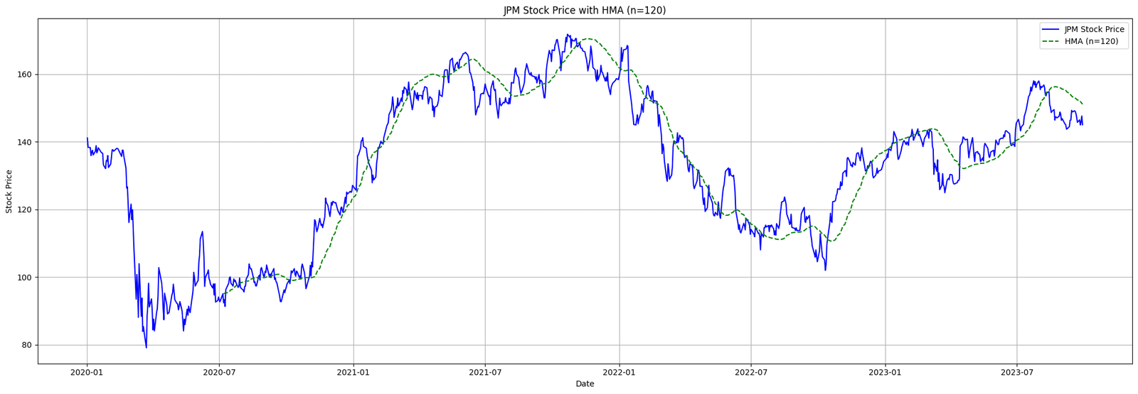
Figure. 9: JPMorgan Chase & Co. (JPM) Stock Price with its 120-day Hull Moving Average (HMA) from 2020 to 2023, illustrating the HMA’s ability to capture the underlying trend while reducing lag and noise.
3. Adaptive and Dynamic
3.1 Fractal Adaptive Moving Average (FRAMA)
FRAMA (Fractal Adaptive Moving Average) is a moving average that takes into account market volatility and adapts its speed accordingly. The core idea behind FRAMA is that markets, like fractals, have similar patterns on both small and large scales.
By determining the fractal dimension of a price series, the FRAMA adjusts its sensitivity, becoming faster during trending periods and slower during sideways movements.
The metdholody for FRAMA is slightly more complex for as it involves computing the fractal dimension.
At a high-level, FRAMA is calculated using the following steps:
- Split the data into two batches.
- Calculate the ’N’ value (difference between the maximum and minimum) for both batches.
- Determine the combined ’N’ value for the two batches.
- Compute the fractal dimension using the ’N’ values.
- Calculate the adaptive filter factor (alpha) using the fractal dimension.
- Compute the FRAMA value using the alpha value and the price data.
The basic structure of the mathemtical representation is the following:
N(t) determines the adaptive window length of the FRAMA based on the price series’ fractal nature.

α(t) defines the FRAMA’s sensitivity by adjusting its response to recent price changes.
FRAMA(t) calculates the adaptive moving average value using the fractal dimension of the market.
Where:
- D(t) is the fractal dimension.
- N(t) is the adjusted dimension.
- α(t) is the weighting multiplier.
- P(t) is the price at time t.
Application
The key aspect of FRAMA is the adaptive filter factor, which determines the sensitivity of the moving average. A higher fractal dimension leads to a more reactive moving average, while a lower dimension results in a smoother curve.
FRAMA can be used similarly to other moving averages, such as identifying trends and generating buy/sell signals. A notable advantage of FRAMA over traditional moving averages is its adaptive nature, which can be more responsive to significant price changes.
When the price is trending, FRAMA can shorten its period, making it more responsive to price changes. Conversely, during sideways or non-trending periods, FRAMA can lengthen its period, providing a smoother line that’s less prone to false signals.
					import yfinance as yf
import numpy as np
import matplotlib.pyplot as plt

def fetch_data(ticker_symbol, start_date, end_date):
    data = yf.download(ticker_symbol, start=start_date, end=end_date)
    return data

def calculate_FRAMA(data, batch=10):
    # Input
    InputPrice = data['Close'].values

    Length = len(InputPrice)
    Filt = np.array(InputPrice)

    # Sequentially calculate all variables and the output
    for i in range(2 * batch, Length):

        # Take 2 batches of the input
        v1 = InputPrice[i-2*batch:i - batch]
        v2 = InputPrice[i - batch:i]

        # For the 1st batch calculate N1
        H1 = np.max(v1)
        L1 = np.min(v1)
        N1 = (H1 - L1) / batch

        # For the 2nd batch calculate N2
        H2 = np.max(v2)
        L2 = np.min(v2)
        N2 = (H2 - L2) / batch

        # For both batches calculate N3
        H = np.max([H1, H2])
        L = np.min([L1, L2])
        N3 = (H - L) / (2 * batch)

        # Calculate fractal dimension
        Dimen = 0
        if N1 > 0 and N2 > 0 and N3 > 0:
            Dimen = (np.log(N1 + N2) - np.log(N3)) / np.log(2)

        # Calculate lowpass filter factor
        alpha = np.exp(-4.6 * (Dimen) - 1)
        alpha = np.clip(alpha, 0.1, 1)  # Ensuring alpha stays between 0.1 and 1

        # Filter the input data
        Filt[i] = alpha * InputPrice[i] + (1 - alpha) * Filt[i-1]

    data['FRAMA'] = Filt
    return data

# Fetching data
ticker_symbol = "AMZN"
start_date = "2020-01-01"
end_date = "2024-01-01"
data = fetch_data(ticker_symbol, start_date, end_date)

# Calculating FRAMA
data = calculate_FRAMA(data)

# Plotting
plt.figure(figsize=(20,7))
data['Close'].plot(label="Close Price", color="blue")
data['FRAMA'].plot(label="FRAMA", color="green", alpha=0.7)
plt.title(f"{ticker_symbol} Stock Price and FRAMA")
plt.legend()
plt.grid(True)
plt.show()
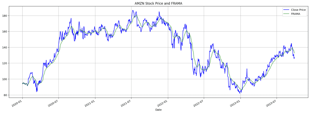
Figure. 10: Visualization of AMZN Stock Price with its FRAMA from 2020 to 2023: The blue line represents the closing price of Amazon (AMZN) stock, while the green line denotes the Fractal Adaptive Moving Average (FRAMA). The FRAMA adapts to market volatility, adjusting its sensitivity to capture price trends and movements.
3.2 Zero Lag Exponential Moving Average (ZLEMA)
The Zero Lag Exponential Moving Average (ZLEMA) is a type of exponential moving average that aims to eliminate the lag associated with traditional EMAs.
The primary goal of ZLEMA is to adjust recent prices to react faster to price changes. It does this by subtracting a lagged EMA from the current price, aiming to provide a faster-moving line with virtually zero lag.
The formula for ZLEMA involves a few steps:
- Calculate the lag: Lag = n / 2, where n is the ZLEMA period.
- Create a new series, Adjusted Close, by subtracting the Lag-day EMA from the close: Adjusted Close = Close − EMA_Lag (Close)
- Calculate ZLEMA: ZLEMA = EMA_n (Adjusted Close).
The ZLEMA’s strength lies in its quest for real-time market reactions. Traditional EMAs, by nature, have an inherent delay; ZLEMA seeks to sidestep this by recalibrating recent prices. By subtracting a lagged EMA, it projects an accelerated response curve that closely trails live price action.
For traders, this offers a distinct advantage: capturing rapid price shifts as they unfold, rather than playing catch-up. This nimbleness can be pivotal in fast-paced markets. Yet, its aggressive responsiveness warrants caution. A keen trader often contrasts ZLEMA’s insights with other indicators to discern genuine trends from fleeting fluctuations.
					import yfinance as yf
import numpy as np
import matplotlib.pyplot as plt

def calculate_EMA(prices, period):
    alpha = 2 / (period + 1)
    EMA = [prices[0]]
    for price in prices[1:]:
        EMA.append((price - EMA[-1]) * alpha + EMA[-1])
    return EMA

def calculate_ZLEMA(prices, period):
    lag = period // 2
    adjusted_prices = [2*prices[i] - (prices[i - lag] if i >= lag else prices[0]) for i in range(len(prices))]
    ZLEMA = calculate_EMA(adjusted_prices, period)
    return ZLEMA

# Fetching data
ticker_symbol = "AAPL"
data = yf.download(ticker_symbol, start="2020-01-01", end="2023-01-01")

close_prices = data['Close'].tolist()

# Calculate ZLEMA
zlema_period = 28
data['ZLEMA'] = calculate_ZLEMA(close_prices, zlema_period)

# Plotting
plt.figure(figsize=(20,7))
plt.plot(data.index, data['Close'], label='Price', color='black')
plt.plot(data.index, data['ZLEMA'], label=f'ZLEMA {zlema_period}', color='red')
plt.title(f'Zero Lag Exponential Moving Average (ZLEMA) of {ticker_symbol} (n = {zlema_period})')
plt.legend()
plt.grid()
plt.show()
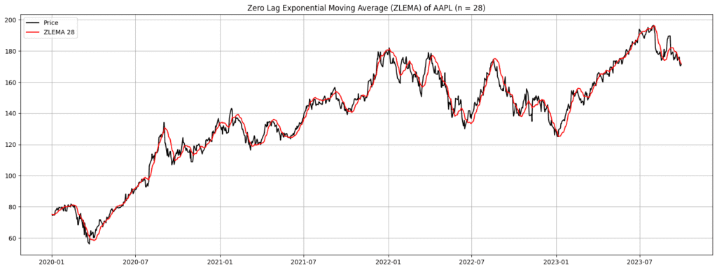
Figure. 11: Zero Lag Exponential Moving Average (ZLEMA) Analysis of AAPL from 2020 to 2023: The graph presents Apple Inc. (AAPL) stock price depicted in black, contrasted with its 28-period ZLEMA in red. The ZLEMA aims to eliminate the lag associated with traditional EMAs, providing a potentially more timely representation of the stock’s trend.
3.3 Variable Index Dynamic Average (VIDYA)
VIDYA, or Variable Index Dynamic Average, is an adaptive moving average introduced by Tushar Chande in the early 1990s. The fundamental idea behind VIDYA is to adjust the smoothing constant dynamically based on the volatility of the price series.
By doing so, VIDYA can respond faster in volatile markets and slow down in trending markets. The rate of adjustment is governed by a volatility index, with the Chande Momentum Oscillator (CMO) often being the chosen index for this purpose.
The VIDYA is calculated as:
VIDYA(t), an adaptive moving average that adjusts its smoothing constant based on price volatility, using the Chande Momentum Oscillator (CMO) as its volatility index
Where:
- VIDYAt is the VIDYA at time t.
- VIDYA_t−1 is the VIDYA at time t−1.
- ABS(CMO_t) is the absolute value of the Chande Momentum Oscillator at time t, scaled between 0 and 1.
- Close_t is the close price at time t.
VIDYA is an adaptive moving average tailored for fluctuating markets. It dynamically adjusts its sensitivity based on market volatility, quickening during turbulence and slowing in steadier periods.
					import yfinance as yf
import numpy as np
import matplotlib.pyplot as plt

def calculate_CMO(prices, period):
    """ Calculate Chande Momentum Oscillator (CMO) """
    deltas = np.diff(prices)
    sum_gains = np.cumsum(np.where(deltas >= 0, deltas, 0))
    sum_losses = np.abs(np.cumsum(np.where(deltas < 0, deltas, 0)))

    cmo = 100 * (sum_gains - sum_losses) / (sum_gains + sum_losses)
    return np.insert(cmo, 0, 0)  # Add a zero at the beginning for alignment

def calculate_VIDYA(prices, period):
    cmo_values = calculate_CMO(prices, period)
    vidya = [prices[0]]

    for i in range(1, len(prices)):
        alpha = abs(cmo_values[i]) / 100  # Normalize CMO to [0, 1]
        vidya.append((1 - alpha) * vidya[-1] + alpha * prices[i])

    return vidya

# Fetching data
ticker_symbol = "V"
data = yf.download(ticker_symbol, start="2020-01-01", end="2024-01-01")
close_prices = data['Close'].tolist()

# Calculate VIDYA
vidya_period = 14
data['VIDYA'] = calculate_VIDYA(close_prices, vidya_period)

# Plotting
plt.figure(figsize=(20,7))
plt.plot(data.index, data['Close'], label='Price', color='black')
plt.plot(data.index, data['VIDYA'], label=f'VIDYA {vidya_period}', color='blue')
plt.title(f'Variable Index Dynamic Average (VIDYA) of {ticker_symbol} (n = {vidya_period})')
plt.legend()
plt.grid()
plt.show()
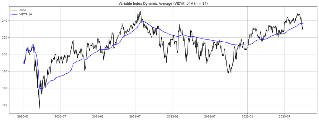
Figure. 12: Variable Index Dynamic Average (VIDYA) Analysis of Visa Inc. (V) from 2020 to 2023: The graph showcases Visa Inc.’s (V) stock price illustrated in black, with its 14-period VIDYA depicted in blue. VIDYA, a dynamic exponential moving average, adjusts its sensitivity based on the Chande Momentum Oscillator (CMO) to better capture volatile market conditions and provide timely insights.
3.4 Arnaud Legoux Moving Average (ALMA)
The Arnaud Legoux Moving Average (ALMA) was developed by Arnaud Legoux and Dimitris Kouzis-Loukas to try to minimize the lag associated with traditional moving averages and make the moving average more responsive to recent price changes while also remaining smooth.
The ALMA uses a sliding window approach and weights the data with a Gaussian function, ensuring the most recent prices have a higher weight.
To calculate the ALMA for a period n, we can use the following formula:

The Arnaud Legoux Moving Average (ALMA): A responsive moving average that leverages a Gaussian weighting scheme to give more significance to recent prices.
Where:
- Price_t−n+i+1 is the price at the time t−n+i+1.
- wi is the weight of the ith data point in the window and is calculated as:

Weight in ALMA: Uses the Gaussian function to determine the weight for each data point based on its position in the window, emphasizing recent prices.
Where:
- moff is n−1/2 offset by the parameter offset.
- σ is n / 6 which defines the width of the Gaussian window.
Application
By harnessesing the power of a Gaussian function within a sliding window ensures that recent prices command higher significance, resulting in a moving average that swiftly acknowledges contemporary price shifts, all while maintaining a commendable smoothness.
For traders on the hunt for a finely-tuned blend of immediacy and clarity, the ALMA offers a compelling proposition. However, as always, it’s prudent to use ALMA readings with other technical metrics for a holistic market analysis.
					import yfinance as yf
import numpy as np
import matplotlib.pyplot as plt

def calculate_ALMA(prices, period, offset=0.85, sigma=6):
    m = np.floor(offset * (period - 1))
    s = period / sigma
    alma = []

    for i in range(period - 1, len(prices)):
        weights = [np.exp(- (j - m)**2 / (2 * s * s)) for j in range(period)]
        sum_weights = sum(weights)
        normalized_weights = [w/sum_weights for w in weights]

        window = prices[i-period+1:i+1]
        alma_value = sum([normalized_weights[j] * window[j] for j in range(period)])
        alma.append(alma_value)

    return [None]*(period-1) + alma  # Pad the beginning with None for alignment

# Fetching data
ticker_symbol = "BABA"
data = yf.download(ticker_symbol, start="2020-01-01", end="2024-01-01")
close_prices = data['Close'].tolist()

# Calculate ALMA
alma_period = 36
data['ALMA'] = calculate_ALMA(close_prices, alma_period)

# Plotting
plt.figure(figsize=(20,7))
plt.plot(data.index, data['Close'], label=f'{ticker_symbol} Price', color='black')
plt.plot(data.index, data['ALMA'], label=f'ALMA {alma_period}', color='purple')
plt.title(f'Arnaud Legoux Moving Average of {ticker_symbol} (n = {alma_period})')
plt.legend()
plt.grid()
plt.show()
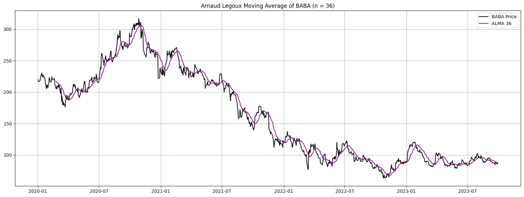
Figure. 13: Arnaud Legoux Moving Average (ALMA) of Alibaba Group (BABA) from 2020 to 2023: The chart displays BABA’s stock price (black line) alongside its 14-day ALMA (purple line), highlighting the trend and smoothing out price fluctuations.
3.5 MESA Adaptive Moving Average (MAMA) and Following Adaptive Moving Average (FAMA)
The MESA Adaptive Moving Average (MAMA) emerged from the forward-thinking of John Ehlers, spotlighted in his work “Cybernetic Analysis for Stocks and Futures.” Rooted in the Maximum Entropy Spectral Analysis (MESA) approach, MAMA was conceived to dynamically tackle non-stationary data, like fluctuating stock prices, which might possess evolving statistical properties.
Traditional averages, no matter their typology, often lag during periods of heightened volatility. MAMA’s hallmark is its adaptability to price volatility. During abrupt price variations, MAMA springs into action, offering near-instantaneous reflections of market movements. Conversely, in periods of stable price trends, its adaptability moderates its pace, curating a clearer depiction of genuine price trends by filtering out market noise.
Complementing MAMA is the Following Adaptive Moving Average (FAMA), which magnifies changing market trends. As a derivative of MAMA, FAMA illuminates areas prone to price corrections within trending markets. Such insights are pivotal for demarcating the culmination of correction phases and the likely resurgence of the prevailing trend.
Formulas and Derivations are as follows:
MESA Adaptive Moving Average (MAMA):
Deriving from MESA and the Hilbert Transform, MAMA’s adjustability is anchored to the calculation of the dominant cycle period. At its core:
- The raw price phase is ascertained using the Hilbert Transform.
- An instantaneous period is deduced, which inversely relates to the instantaneous frequency.
- This instantaneous period is smoothed to unveil the dominant cycle period.
- The dominant cycle period is then leveraged to compute the smooth price.
The ensuing MAMA value mirrors an adaptive average resonating with recent price dynamics.
Following Adaptive Moving Average (FAMA):
FAMA underscores trend inflection points. Its essence can be captured by:
Formula for the Following Adaptive Moving Average (FAMA). The equation describes how FAMA at any given time (FAMAt) is computed based on its previous value (FAMAt−1), the current price, and an adaptive smoothing constant (α), which is derived from MAMA.
Where:
- α is the adaptive smoothing constant, a byproduct of MAMA.
Application
Consider a stock price demonstrating a consistent uptrend interspersed with minor fluctuations. Here, MAMA traces this ascent smoothly, adeptly filtering minor noise. Simultaneously, FAMA, with its heightened sensitivity, mirrors the short-term deviations around MAMA, hinting at possible correction points.
Suddenly, a market-altering news event precipitates a sharp price drop. MAMA, with its adaptive nature, aligns quickly with this price transformation. The more reactive FAMA might cross MAMA, a potential bearish signal for traders.
Post this upheaval, if the stock price finds its footing and commences recovery, MAMA will gracefully track this new trajectory. Concurrently, FAMA will offer granular insights into trend continuities and minor corrections.
					import yfinance as yf
import talib
import matplotlib.pyplot as plt

# Fetching data
ticker_symbol = "GOOGL"
data = yf.download(ticker_symbol, start="2020-01-01", end="2024-01-01")

# Calculating MAMA and FAMA
data['MAMA'], data['FAMA'] = talib.MAMA(data['Close'].values)

# Plotting both MAMA and FAMA
plt.figure(figsize=(20,7))
plt.plot(data.index, data['Close'], label='Price', color='black')
plt.plot(data.index, data['MAMA'], label='MAMA', color='blue')
plt.plot(data.index, data['FAMA'], label='FAMA', color='red')
plt.title(f'MESA Adaptive Moving Average (MAMA) & Following Adaptive Moving Average (FAMA) of {ticker_symbol}')
plt.legend()
plt.grid()
plt.show()
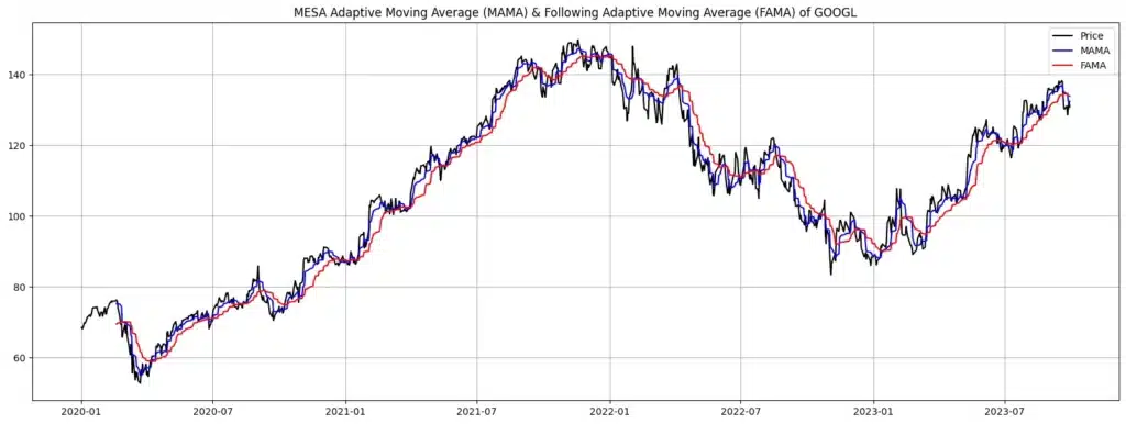
Figure. 14: MESA Adaptive Moving Average (MAMA) and Following Adaptive Moving Average (FAMA) of GOOGL (2020–2023): The combined chart illustrates the relationship between Apple’s stock price, MAMA, and FAMA. By studying the interactions between the stock price and these indicators, traders can discern potential market trend shifts and trading opportunities.
3.6 Adaptive Period Moving Average
The Adaptive Period Moving Average (APMA) adjusts the period of the moving average dynamically based on recent market volatility. When prices are volatile, the APMA shortens its period to be more sensitive to recent price changes.
When prices are less volatile, the APMA lengthens its period to reduce noise and generate smoother signals. The APMA may employ different metrics to measure volatility, like standard deviation or the Average True Range (ATR).
The general idea behind the APMA is to adjust the period of the moving average based on a measure of volatility.
The formula can be expressed as:
Formula for the Adaptive Period Moving Average (APMA). The formula dynamically adjusts the moving average period based on recent market volatility. The Adjusted Period is determined by current volatility in relation to observed maximum and minimum volatilities.
Where:
- Adjusted Period is the calculated period for the moving average based on current volatility.
- Maximum Period and Minimum Period are user-defined constants specifying the bounds of the possible period adjustments.
- Max Volatility and Min Volatility are the maximum and minimum observed volatilities, respectively.
- Current Volatility is the measure of recent volatility, typically calculated using ATR or standard deviation
Note: The above formula is just a possible approach to adjust the moving average period. There can be other methods or variations.
Application
APMA stands out by dynamically calibrating its sensitivity based on market volatility, offering traders a real-time edge. In volatile conditions, its shorter period captures swift price changes, ensuring timely responses.
During stable phases, its lengthened period filters out market noise, yielding cleaner signals. This adaptability not only aids precise trend identification but also enhances risk assessment.
					import yfinance as yf
import numpy as np
import matplotlib.pyplot as plt

def adaptive_period_moving_average(prices, min_period=5, max_period=30):
    atr = np.zeros_like(prices)
    adjusted_periods = np.zeros_like(prices)
    moving_averages = np.full_like(prices, np.nan)  # Initialize with NaN values

    for i in range(1, len(prices)):
        atr[i] = atr[i-1] + (abs(prices[i] - prices[i-1]) - atr[i-1]) / 14

        min_volatility = atr[1:i+1].min()
        max_volatility = atr[1:i+1].max()

        if max_volatility == min_volatility:
            adjusted_period = min_period
        else:
            adjusted_period = int(((max_period - min_period) / (max_volatility - min_volatility)) * (atr[i] - min_volatility) + min_period)

        adjusted_periods[i] = adjusted_period

        if i >= adjusted_period:
            moving_averages[i] = np.mean(prices[i-adjusted_period+1:i+1])

    return moving_averages

# Fetching data
ticker_symbol = "MA"
data = yf.download(ticker_symbol, start="2020-01-01", end="2024-01-01")

data['APMA'] = adaptive_period_moving_average(data['Close'].values)

# Plotting
plt.figure(figsize=(20,7))
plt.plot(data.index, data['Close'], label='Price', color='black')
plt.plot(data.index, data['APMA'], label='Adaptive Period MA', color='red')
plt.title(f'Adaptive Period Moving Average (APMA) of {ticker_symbol}')
plt.legend()
plt.grid()
plt.show()
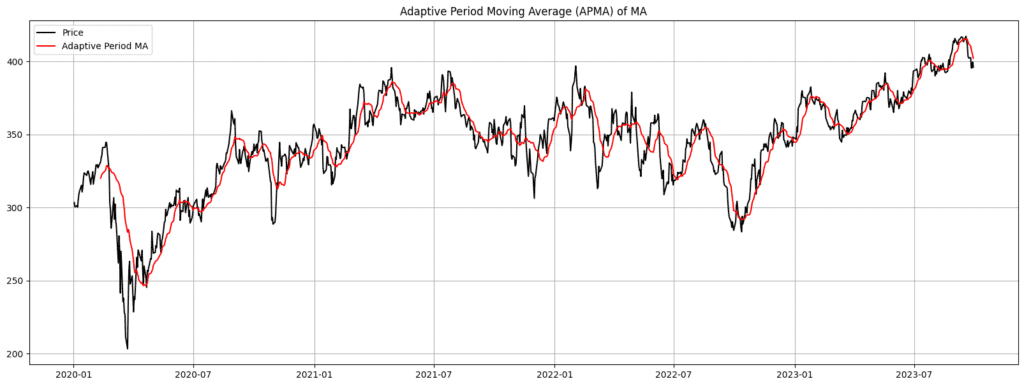
Figure. 15: APMA of MA (2020–2023): The APMA (red) adjusts its period based on price volatility, ranging between a minimum and maximum period. For Mastercard’s stock (black), this technique dynamically alters its sensitivity, providing a flexible smoothing of price trends influenced by the observed volatility.
3.7 Rainbow Moving Average
The Rainbow Moving Average is a collection of exponential moving averages (EMAs) with different periods. It is called “Rainbow” because when plotted, the collection of EMAs resembles the colors of a rainbow, especially when you color-code them in a spectrum.
The Rainbow Moving Average helps to visualize the convergence and divergence of short-term and long-term trends. When the EMAs are intertwined or braided, it indicates a lack of trend or a weak trend. When the EMAs separate, with shorter periods on top and longer periods at the bottom (or vice versa), it indicates a stronger trend.
Computational Formula for the Exponential Moving Average (EMA) with Smoothing Factor.
- EMAt is the Exponential Moving Average for the current time t
- Pt is the price for the current time t
- α is the smoothing factor, calculated as α = 2 / (N+1)
- N is the period of the EMA
- EMAt−1 is the Exponential Moving Average for the previous time t−1
Application
Given its layered structure, traders can easily gauge the relative strength of different timeframes at a glance. For instance, if longer-term EMAs shift above shorter ones, it could signify a potential reversal, moving from a bullish to bearish sentiment. Additionally, the RMA acts as a dynamic support and resistance mechanism; prices may often rebound or face resistance around these moving average lines.
By assessing the distance between individual EMAs in the RMA, traders can also gauge market volatility. A wider spread might indicate heightened volatility, while a narrower spread can suggest a more stable environment. In essence, the RMA provides a consolidated lens through which traders can evaluate multiple market dimensions simultaneously.
					import yfinance as yf
import matplotlib.pyplot as plt

# Download stock data
ticker = "NVDA"
data = yf.download(ticker, start="2020-01-01", end="2023-12-26")
# Calculate EMAs with different lookback periods
lookback_periods = [2, 4, 8, 16, 32, 64, 128, 192, 320, 512]
colors = ['red', 'orange', 'yellow', 'green', 'blue', 'indigo', 'violet', 'black','gray','brown']
for i, lookback in enumerate(lookback_periods):
    data[f'EMA{lookback}'] = data['Close'].ewm(span=lookback).mean()
# Plot the results
plt.figure(figsize=(20,7))
plt.plot(data['Close'], label='Close', linewidth=2, alpha=0.8, color='black')
for i, lookback in enumerate(lookback_periods):
    plt.plot(data[f'EMA{lookback}'], label=f'EMA {lookback}', linewidth=1.5, alpha=0.8, color=colors[i])
plt.title(f'{ticker} Rainbow Moving Average')
plt.xlabel('Date')
plt.ylabel('Price')
plt.legend()
plt.grid()
plt.show()
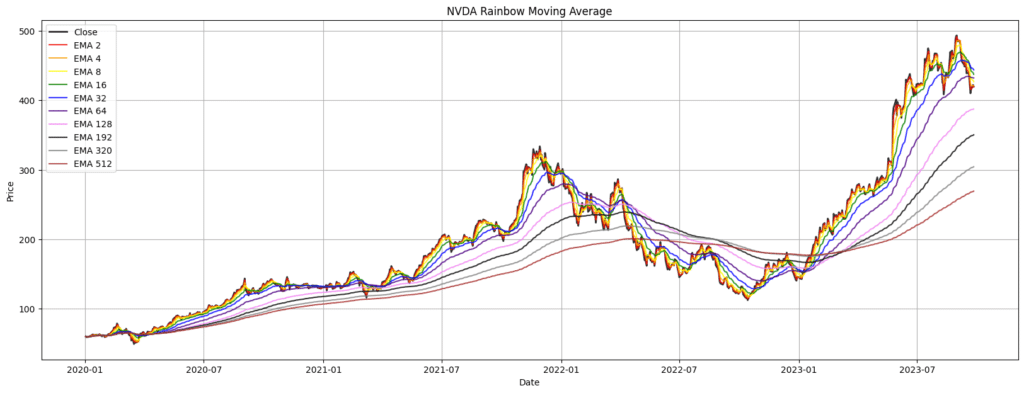
Figure. 16: Rainbow Moving Average for NVIDIA (NVDA) (2020–2023): The graph displays NVDA’s stock price alongside EMAs with varying lookback periods. Each EMA is depicted in a distinct color, from short (red) to long-term (brown) trends, offering a multi-layered view of price movements.
3.8 Wilders Moving Average
The Wilders Moving Average is a special type of exponential moving average developed by J. Welles Wilder, the author of the book “New Concepts in Technical Trading Systems.” This average was primarily designed for commodity and stock markets to measure the volatility of price movements.
The Wilders Moving Average places more weight on past prices compared to the regular exponential moving average, making it react more slowly to recent price changes. This characteristic of the Wilders MA makes it particularly useful for trending markets, as it reduces the noise of minor price fluctuations.
The Wilders Moving Average formula:
Formula for the Wilders Moving Average (WMA). Developed by J. Welles Wilder, this unique exponential moving average emphasizes past prices more than traditional EMAs. WMAt represents the Wilders Moving Average at time t, calculated based on the close price (Ct) and a specified lookback period (N).
Where:
- WMAt is the Wilders Moving Average at time t.
- Ct is the close price at time t.
- N is the lookback period.
This formula is similar to the EMA, but the weighting is different. By prioritizing past prices, it provides a steady and less volatile representation of market sentiment, reducing susceptibility to short-term price shocks.
This focus enhances interpretability, allowing traders to discern more sustained market trends and minimize the influence of transient fluctuations.
					import yfinance as yf
import pandas as pd
import matplotlib.pyplot as plt

def wilders_moving_average(prices, period):
    wilder = [prices[0]]
    for price in prices[1:]:
        wilder_value = ((wilder[-1] * (period - 1)) + price) / period
        wilder.append(wilder_value)
    return wilder

# Fetching data
ticker_symbol = "AAPL"
data = yf.download(ticker_symbol, start="2020-01-01", end="2024-01-01")

# Calculate Wilders Moving Average
period = 14
data['Wilders_MA'] = wilders_moving_average(data['Close'].tolist(), period)

# Plotting
plt.figure(figsize=(20,7))
plt.plot(data.index, data['Close'], label='Price', color='black')
plt.plot(data.index, data['Wilders_MA'], label=f'Wilders MA {period}', color='red')
plt.title(f'Wilders Moving Average of {ticker_symbol} (n = {14})')
plt.legend()
plt.grid()
plt.show()

Figure. 17: Wilder’s Moving Average of AAPL (2020–2023): This chart displays Apple’s stock price alongside Wilder’s Moving Average, a method emphasizing earlier price data. The comparison offers insights into potential market trends.
3.9 Smoothed Moving Average (SMMA)
The Smoothed Moving Average (SMMA) is a type of moving average that takes into account a vast amount of data points, smoothing out fluctuations in the data to provide a clearer view of the underlying trend.
Unlike the Simple Moving Average (SMA) and the Exponential Moving Average (EMA), the SMMA gives equal weight to all prices in its series.
The SMMA is calculated as follows:
For the first period:
Initial calculation for the Smoothed Moving Average (SMMA). This equation outlines the method for determining the initial value of the SMMA, providing the foundation for subsequent computations. Unlike other moving averages, SMMA assigns equal significance to all prices within its series.
For subsequent periods:
Subsequent calculation for the Smoothed Moving Average (SMMA) for periods after the first. SMMAi denotes the Smoothed Moving Average for the current period, and Pricei is the asset’s price at that period. The period of the SMMA is represented by n.
- SMMAi is the Smoothed Moving Average for the current period.
- Pricei is the price of the asset at the current period.
- n is the period of the SMMA.
Application
When the price hovers around the SMMA, it can signify a consolidative or range-bound market, where neither the bulls nor the bears have definitive control.
Sudden departures from the SMMA can also signify breakout moments, either upward or downward. By analyzing the proximity and movement of the price relative to the SMMA, traders can deduce potential future price directions and adjust their strategies accordingly.
					import yfinance as yf
import matplotlib.pyplot as plt

def calculate_SMMA(prices, n):
    SMMA = [np.nan] * (n-1)  # Fill the initial n-1 values with NaN
    SMMA.append(sum(prices[:n]) / n)
    for i in range(n, len(prices)):
        smma_value = (SMMA[-1] * (n - 1) + prices[i]) / n
        SMMA.append(smma_value)
    return SMMA

# Fetching data
ticker_symbol = "VOW.DE"
data = yf.download(ticker_symbol, start="2020-01-01", end="2024-01-01")

# Calculate SMMA
n = 28
data['SMMA'] = calculate_SMMA(data['Close'].tolist(), n)

# Plotting
plt.figure(figsize=(20,7))
plt.plot(data.index, data['Close'], label='Price', color='black')
plt.plot(data.index, data['SMMA'], label=f'SMMA {n}', color='red')
plt.title(f'Smoothed Moving Average (SMMA) of {ticker_symbol} (n ={n})')
plt.legend()
plt.grid()
plt.show()
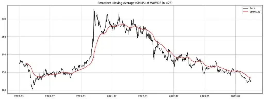
Figure. 18: Smoothed Moving Average (SMMA) of VOW.DE (2020–2023): The SMMA provides a smoothing effect by placing equal weight on every price, thus minimizing volatility. Over a 14-day period, the chart contrasts Volkswagen’s stock price (black) with its 28-day SMMA (red), highlighting a gentler curve that offers a clearer picture of price trends.
Related Articles
The Art of Crossing Over Moving Averages in Python

Newsletter
One thought on “Top 36 Moving Averages Methods For Stock Prices in Python”