Experience the Future of Intelligent Investing Today
Back To Top
Experience the Future of Intelligent Investing Today
Instead of merely allocating assets based on potential returns or market capitalization, Risk Parity Rebalancing emphasizes creating a harmonious balance where each asset contributes equally to a portfolio’s overall risk. The goal? Deliver consistent returns while taming the unruly beast of market volatility.
Traditionally, many investors favored a 60/40 stock-bond split for a balanced growth and security blend. However, as financial markets grew more complex, the appeal of sophisticated strategies like Risk Parity surged. This method ensures that each asset, or its group, equally influences the portfolio’s overall risk, preventing disproportionate sway.
The theoretical appeal of Risk Parity Rebalancing is undeniable, but its real-world applications further cement its reputation in the investment community. A few prominent instances include:
Risk Parity, with its emphasis on holistic risk management, offers a compelling answer to this age-old conundrum. In the sections that follow, we’ll delve deeper into the mathematical underpinnings of Risk Parity, its Python-based implementation, and further insights into its application, performance, and potential future.
Risk Parity is an investment approach where the goal is to allocate capital based on risk, rather than on returns or other criteria. The primary objective is to achieve a balanced portfolio where each asset contributes equally to the overall risk. By doing this, the strategy seeks to enhance portfolio diversification and, ideally, achieve more consistent returns over time.
At its core, Risk Parity is about balance. Traditional investment strategies often rely on expected returns to determine asset allocation, but this can lead to concentrated risks in certain assets. For instance, even in a diversified portfolio, equities might represent a disproportionate amount of risk, especially when market conditions are volatile.

Equation. 1: The formula for calculating the inverse volatility weights in Risk Parity.
Where:
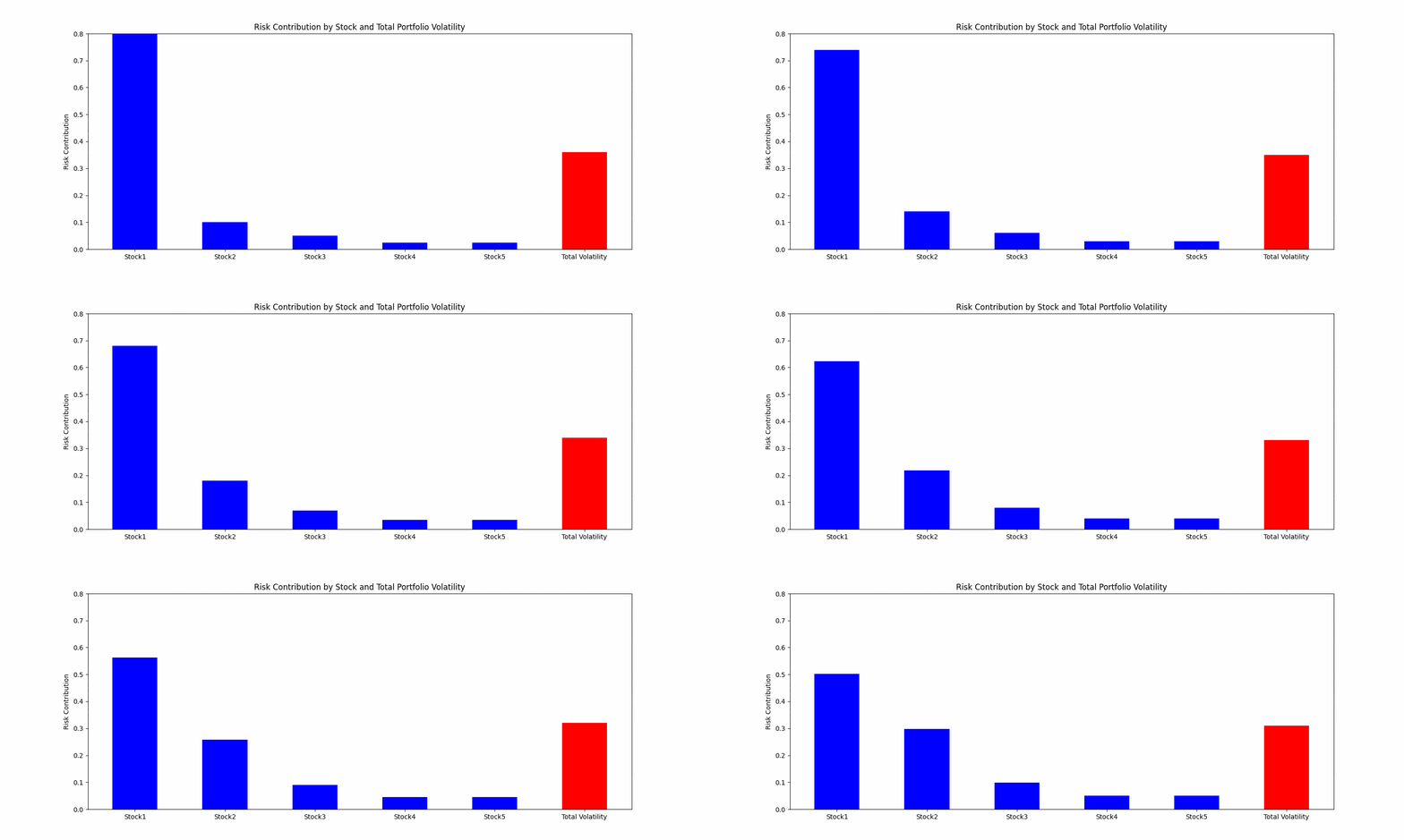
Simply put, assets with lower volatility are given higher portfolio weights, and vice versa. The goal is to balance out the risk contributions of each asset:

Figure. 1: Visualizing Risk Parity: as Individual stock risk contributions adjust dynamically, observe how the total portfolio volatility responds in tandem, showcasing the essence of risk balanced asset allocation.
Risk Parity isn’t a magic bullet, and like all strategies, it has its strengths and potential pitfalls. On the upside, it provides a more balanced portfolio, potentially leading to steadier returns, especially during tumultuous market periods. On the flip side, the strategy might require the use of leverage to achieve desired returns, which can amplify both gains and losses.
This section will illustrate how one can utilize Python to fetch stock data, compute Risk Parity weights, simulate a Risk Parity portfolio, and visualize the performance results.
Before we jump into the code, ensure you have the required libraries installed. Our analysis leans on a few essential Python packages:
					# Fetch stock data directly from Yahoo Finance.
import yfinance as yf

# For data manipulation and analysis.
import pandas as pd

# Used for mathematical operations.
import numpy as np

# Essential for data visualization.
import matplotlib.pyplot as plt
Our starting point is to acquire the historical data for our selected assets and a benchmark index:
					def fetch_returns(tickers):
    data = yf.download(tickers + ['^GSPC'], start="2010-01-01", end="2023-01-01")['Adj Close']
    return data.pct_change().dropna()
Here, fetch_returns fetches the adjusted closing prices for our tickers and the S&P 500 (our benchmark), calculates daily returns, and cleans up any NA values.
The essence of Risk Parity lies in balancing risk contributions across assets:
					def calculate_weights(data):
    vol = data.rolling(window=60).std().dropna().iloc[-1][:-1]  # Exclude S&P 500 index
    inv_vol = 1 / vol
    weights = inv_vol / np.sum(inv_vol)
    return weights
In calculate_weights, we calculate the rolling 60-day volatility for each asset, derive the inverse volatilities, and normalize them to obtain the Risk Parity weights.
Simulating the Risk Parity portfolio’s performance over time:
					def simulate_portfolio(returns, n_days=60):
    port_val = [1]
    sp500_val = [1]
    weights = np.ones(len(tickers)) / len(tickers)  # Start with equal weights

    for i in range(len(returns)):
        if i < 60:  # If less than rolling window, use equal weights
            daily_port_return = np.dot(returns.iloc[i][:-1], weights)
        else:
            if i % n_days == 0:  # Rebalancing
                weights = calculate_weights(returns.iloc[i-60:i])
            daily_port_return = np.dot(returns.iloc[i][:-1], weights)

        port_val.append(port_val[-1] * (1 + daily_port_return))
        sp500_val.append(sp500_val[-1] * (1 + returns.iloc[i]['^GSPC']))
    return port_val, sp500_val
The function begins with an equal weightage for all assets. As the simulation progresses, it recalculates the weights based on the Risk Parity principle every n_days. This dynamic adjustment ensures the portfolio remains balanced in terms of risk.
The purpose of any investment strategy is to outperform a benchmark:

Newsletter