Experience the Future of Intelligent Investing Today
Back To Top
Experience the Future of Intelligent Investing Today
Traditionally, we’ve leaned on correlation matrices for understanding inter-asset dynamics. Yet, as market crashes of the past have shown, when the storm hits, many models go haywire. Suddenly, correlations seem to converge to one, and diversification, the oft-touted risk management mantra, appears to offer little refuge.
This unexpected synchronization, where assets move in near-perfect harmony during downturns, has caused leading finance firms and institutional investors to increasingly turn their attention to more sophisticated tools to analyze the tail of asset distributions. This is where copulas come into play. These tools, moving beyond simplistic correlation, offer a nuanced understanding of asset dependencies, especially during those tumultuous times when markets plunge into chaos.

The core of any risk management model lies in its capacity to grasp the intricate patterns and dependencies between various assets in a portfolio. The richer the understanding, the better equipped we are to handle market upheavals.
Copulas, part of stochastic modeling, capture the dependence structure between random variables without altering their individual behaviors. Moreover, they act as bridges, connecting the behaviors of assets, and allowing a deeper study of their joint movement.
Furthermore, this understanding is critical for financial analysis and risk management. While standard correlation captures linear relationships, it can be blind to intricate dependencies in extreme market conditions. In times when assets show tail dependence, copulas provide a more comprehensive insight into these dynamics.
Copulas stems from multivariate probability theory. Let’s dive into a basic mathematical understanding:
A copula: C:[0,1]^2 → [0,1] is a multivariate cumulative distribution function (CDF) whose one-dimensional margins are uniform on [0, 1], where U and V are random variables with uniform distributions on [0, 1]:

Equation. 1: Defining the joint distribution of U and V using copulas

Equation. 1: Expressing joint distribution H in terms of marginal distributions F and G using a copula
This theorem underscores the beauty of copulas: the ability to separate the dependence structure from the margins. To put it simply, imagine you’re building a house. The margins are like the foundational pillars of the house, while the copula is the blueprint that dictates how these pillars are connected. No matter what materials (marginal distributions) you use for the pillars, the blueprint (copula) remains consistent in connecting them.

Figure. 1: Transitioning from independent stock returns to a dependence structure defined by the Gaussian copula, alongside the dynamic evolution of their correlation. The histograms depict the distribution of stocks A and B throughout the transformation process.
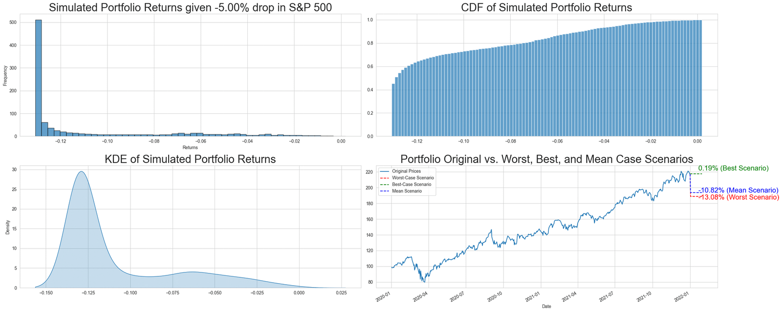
Scenario modelling in finance simulates potential future outcomes based on assumptions, aiding in understanding investment sensitivities to market shifts. The provided code examines how a hypothetical portfolio might react to a significant S&P 500 drop.
We build a hypothetical portfolio consisting of three major tech stocks and retrieve the data yfinance :
					portfolio_tickers = ["MSFT", "AAPL", "GOOGL"]
end_date = "2022-01-01"
start_date = "2020-01-01"
symbols = ["^GSPC"] + portfolio_tickers
data = yf.download(symbols, start=start_date, end=end_date)["Adj Close"]
To ensure that the data is suitable for copula analysis, it needs to lie within a [0,1] range. Quantile transformation is applied, which essentially ranks the data in a uniform distribution.
					for symbol in returns.columns:
    qt = QuantileTransformer(output_distribution='uniform')
    data_uniform[symbol] = qt.fit_transform(returns[[symbol]]).flatten()
    quantile_transformers[symbol] = qt
Given that our primary interest is to understand how a certain drop in the S&P 500 would affect our portfolio stocks, we need to establish a joint behavior between the S&P 500 and each stock. This relationship is captured using a bivariate Gaussian copula.
Using the copula, a conditional distribution is derived, which tells us about the potential behavior of our stocks’ returns, given a certain drop in the S&P 500. This is achieved via the conditional_sample function.
					def conditional_sample(u1, rho, n_samples=1000):
    u2 = np.linspace(0.001, 0.999, n_samples)
    return u2, norm.cdf((norm.ppf(u1) - rho * norm.ppf(u2)) / np.sqrt(1 - rho**2))
For each of the portfolio’s stocks, given the drop in the S&P 500 (specified as a percentage), the copula model is used to simulate potential stock returns. These simulated returns provide insights into probable worst-case, best-case, and mean scenarios for each stock.
					results = {}
for ticker in portfolio_tickers:
    index_drop = quantile_transformers["^GSPC"].transform(np.array([[market_drop_percentage]]))[0][0]

    # Bivariate assumption with ^GSPC and each stock
    bi_data = data_uniform[["^GSPC", ticker]]
    bi_copula = GaussianCopula(dim=2)
    bi_copula.fit(bi_data.values)
    rho = bi_copula.params[0]

    conditional_u2, conditional_cdf = conditional_sample(index_drop, rho)
    conditional_returns = quantile_transformers[ticker].inverse_transform(conditional_cdf.reshape(-1, 1)).flatten()
    results[ticker] = conditional_returns
Putting all the above together, we get the following Python code:

Newsletter