Rank OTM put and call spreads by expected value, probability of profit, IV, delta and pricing in Python.
Selling options can be a profitable avenue, if you know which spreads to sell and how to limit your risk.
Every day, 1000s of puts and calls flash attractive premiums, but either they expire worthless or blow past your risk limits when the market snaps.
Selling credit spreads looks simple. In practice, it’s a minefield: which expiry, which strikes, how wide, what credit, and how much risk is really on the table?
You need more than intuition. You need a system that ranks every possible spread by real, risk-adjusted edge.
We present a scanning system that places probability of profit, expected value, volatility, and liquidity at the center of every spread decision.
The complete Python notebook for the analysis is provided below.
This article is structured as follows:
- The Credit Spread Options Strategy
- Automating the Scanning of Credit Spreads
- Implementing the Scanner in Python
- Using the Scanner in Practise
1. The Credit Spread Options Strategy
A credit spread combines two options: you sell one and buy another at a different strike, same type and expiry. This generates a net premium.
Why buy the second option?
Buying the further out-of-the-money option caps your risk. It creates a defined maximum loss, no matter how far the market moves against you.
Construction
Put credit spread (bull put):
- Sell a put at strike K1
- Buy a put at lower strike K2 (so that K2<K1)
Call credit spread (bear call):
- Sell a call at strike K1
- Buy a call at higher strike K2 (so that K2>K1)
Key Metrics
Net Credit (Premium Collected):
Maximum Loss (Capped):

Break-Even Price:
- Puts: K1−Credit
- Calls: K1+Credit
Return on Risk:
You profit if the underlying finishes above (put spread) or below (call spread) the short strike at expiry.
Losses stop at the maximum loss amount, regardless of market extremes.
Figure 1. Net payoff at expiry for two credit spread strategies: Bull Put (left): short 95 put, long 90 put, net credit $2.00. Bear Call (right): short 105 call, long 110 call, net credit $1.80. Both have capped loss and defined break-even points.
2. Automating the Scanning of Credit Spreads
You can’t manually sift through thousands of option spreads combinations and expect to consistently pick out the best one.
The market moves too fast. Most option sellers need a systematic way to surface only the most favorable trades.
The scanner works by computing the real risk, reward, and probability metrics for every liquid credit spread.
The goal is flag the small subset that offers a risk-adjusted advantage.
What makes a spread worth selling?
It’s not just the premium. You need to know the capital at risk, the odds of a win, and how that edge holds up after liquidity and volatility filters.
Core Metrics and How They Are Calculated:
- Width: This is the distance between your short and long strikes.
- Credit: The net premium collected for selling the spread.
- Max Loss: The maximum you can lose if the spread moves fully against you.
-
- Break-even: The price where profit flips to loss. For puts:

- Return on Risk:

- Probability of Profit (POP): Approximated by delta or calculated with Black-Scholes d₂:
- Expected Value (EV):
- EV per Risk:
- Net Vega, Net Theta: Each spread’s sensitivity to volatility and time.
You need these numbers on every possible combination, every expiry, every width.
That’s why this is a job for code, not a spreadsheet.
Here’s the workflow, step by step:
3. Implementing the Scanner in Python
The code below will (i) fetch live options data, (ii) enrich each strike with implied volatility and Greeks estimates, and (iii) constructs every possible out-of-the-money put or call credit spread combination.
We also calculate a robust set of risk and reward metrics for each combination. We can then sort, filter, and visualize the entire opportunity set.
3.1 Adjust Key Parameters
Set your core variables at the top. Pick your ticker, option type, expiry window, and minimum liquidity.
Each parameter is further explained as a comment in the code snippet below.
These settings filter out illiquid, stale, or mispriced options and focus the scan on real tradable spreads.
import yfinance as yf
import pandas as pd
import numpy as np
from datetime import datetime, timedelta
from math import log, sqrt, exp
from scipy.stats import norm
import plotly.express as px
import matplotlib.pyplot as plt
plt.style.use('dark_background')
# ─── PARAMETERS
TICKER = '^SPX' #"^XSP" # underlying symbol (e.g. "^XSP" or "SPY"); changing this points the scanner at a different market
OPTION_TYPE = "put" # "put" or "call"; switches between scanning put-credit spreads (OTM puts) and call-credit spreads (OTM calls)
MIN_DTE = 1 # minimum days to expiry; ↑ to avoid very short-dated (low gamma, little time decay), ↓ to include them
MAX_DTE = 90 # maximum days to expiry; ↑ to scan far-out expiries (higher extrinsic value), ↓ to focus on near-term
N_STD = 1.0 # threshold in standard deviations for a price “safety” band; ↑ widens the band (more conservative), ↓ tightens it
RISK_FREE = 0.04 # annual risk-free rate used in Black–Scholes; update to current rates—has a small effect on theoretical pricing
MIN_OI = 100 # minimum open interest; ↑ to require more liquid strikes (fewer legs), ↓ to include less-traded strikes
MIN_VOL = 20 # minimum volume today; ↑ to filter stale or inactive strikes, ↓ to accept lower-volume legs
LAST_N_DAYS = 5 # only include options last traded within this many calendar days; ↓ to require fresher trading prints, ↑ to allow older
MAX_SPREAD_PCT = 0.05 # maximum acceptable bid–ask width as a fraction of strike (e.g. 0.1 = 10%); ↓ for tighter pricing, ↑ to allow wider markets
POP_METHOD = "POP" # "delta" uses |Δ| (for calls) or 1−|Δ| (for puts) as approximate POP; "d2" uses Φ(d₂) from B–S for theoretical POP
PRICING_METHOD = "mid" # "mid" uses midpoint pricing for credit; "worst" uses bid for the short leg and ask for the long leg (more conservative)
3.2 Black-Scholes Helper Functions
We now define all pricing and Greek calculations in helper functions. We use standard Black-Scholes formulas.
These functions calculate the theoretical price of each option and extract the risk measures: delta, gamma, theta, and vega.
Each strike also gets an implied volatility estimate based on current market prices. Implied volatility is solved numerically.
These metrics essentially drive the probability, edge, and risk calculations for every spread in the scan.
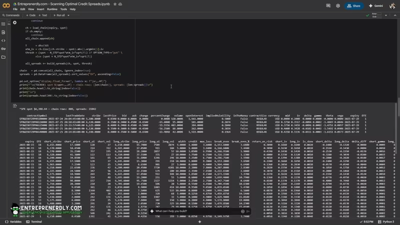
# ─── BLACK–SCHOLES HELPER FUNCTIONS
def _d1(S,K,T,r,σ):
return (log(S/K)+(r+0.5*σ*σ)*T)/(σ*sqrt(T)) if (σ>0 and T>0) else np.nan
def _d2(S,K,T,r,σ):
d1 = _d1(S,K,T,r,σ)
return d1 - σ*sqrt(T) if not np.isnan(d1) else np.nan
def bs_price(S,K,T,r,σ,kind):
d1, d2 = _d1(S,K,T,r,σ), _d2(S,K,T,r,σ)
if np.isnan(d1) or np.isnan(d2):
return np.nan
if kind=="call":
return S*norm.cdf(d1) - K*exp(-r*T)*norm.cdf(d2)
else:
return K*exp(-r*T)*norm.cdf(-d2) - S*norm.cdf(-d1)
def implied_vol(mkt_price,S,K,T,r,kind):
σ = 0.2
for _ in range(60):
price = bs_price(S,K,T,r,σ,kind)
if np.isnan(price):
return np.nan
diff = price - mkt_price
if abs(diff) < 1e-6:
return max(σ,0)
d1 = _d1(S,K,T,r,σ)
vega = S * norm.pdf(d1) * sqrt(T)
if vega < 1e-8:
break
σ -= diff / vega
return np.nan
def greeks(S,K,T,r,σ,kind):
if σ<=0 or T<=0:
return np.nan, np.nan, np.nan, np.nan
d1, d2 = _d1(S,K,T,r,σ), _d2(S,K,T,r,σ)
Δ = norm.cdf(d1) if kind=="call" else norm.cdf(d1)-1
Γ = norm.pdf(d1)/(S*σ*sqrt(T))
V = S*norm.pdf(d1)*sqrt(T)*0.01
if kind=="call":
Θ = (-S*norm.pdf(d1)*σ/(2*sqrt(T))
- r*K*exp(-r*T)*norm.cdf(d2)
)/365
else:
Θ = (-S*norm.pdf(d1)*σ/(2*sqrt(T))
+ r*K*exp(-r*T)*norm.cdf(-d2)
)/365
return Δ, Γ, Θ, V
3.3 Fetch Options Data and Enrich It
Pull the raw chain from yfinance. Filter for volume, open interest, and recent prints.
Compute IV, delta, gamma, theta, and vega for each strike.
Use build_spreads function to pair every valid short leg with a deeper long leg. Filter for realistic pricing.
Then, calculate credit, width, max loss, break-even, POP, EV, and Greek exposures for every spread.
Newsletter