Back To Top

March 13, 2025

Extracting Future Price Expectations from Options

Deriving Risk-neutral Price Forecasts, Estimating Expected Price Distributions and Foward-looking Market Implied Probabilities

Most traders rely on past price movements to predict future trends. But we can actually extract forward-looking prices directly from options prices.

Options prices not only reflect historical volatility but also embed the market’s collective expectations of future prices.

We can construct a forward-looking distribution of expected stock prices based on option-implied probabilities.

This approach goes beyond traditional indicators. It shows where traders believe a stock is most likely to end up by a given expiration date.

In this article, we’ll break down the step-by-step process of deriving market-implied probability distributions using options data. Google Colab Notebook is provided Below.

Use Entreprenerdly’s option-based stock price forecasting tool to get forward-looking price estimates in real time:

Options-Based Price Forecasting With Foward Looking Implied Market Probabilities Demo 2 AVIF
Factor model for exposure and mispricing demo 1 AVIF

In this article, we’ll cover:

  • How to fetch and filter option chain data
  • Calculating implied volatility using the Black-Scholes model
  • Applying the Breeden-Litzenberger formula to extract risk-neutral probabilities
  • Smoothing the probability distribution for better insights
  • Visualizing a 3D implied probability surface over multiple expirations
Figure 4 Implied probability density function for a single expiration. (OPTIMIZED)

1. Extracting Market Expectations from Options

In a risk-neutral world, all assets are expected to grow at the risk-free rate. This assumption allows us to extract implied probabilities directly from option prices. 

The key formula behind this is the Breeden-Litzenberger result, which states that the second derivative of the call price with respect to the strike gives the risk-neutral probability density:

Formula 1 PDF
  • C(K) is the call option price at strike K,
  • r is the risk-free rate,
  • T is the time to expiration.

It allows us to translate market prices into a probability distribution of future stock prices.

Why Implied Volatility Matters

Implied volatility σIV represents market uncertainty about future price movements. 

Unlike historical volatility, which looks backward, implied volatility is forward-looking — it reflects how risky traders expect the stock to be.

The Black-Scholes formula for a European call option captures this:

Formula 2 Call option

d1 is

Formula 3 d1 in bsm

By inverting this formula, we extract implied volatility from market prices and understand how uncertain traders are about the stock’s future.

  • Higher IV = wider probability distribution = greater uncertainty
  • Lower IV = narrower distribution = more confidence in price range

We now have the building blocks:

  1. Option prices → Implied volatilities (market uncertainty)
  2. Implied volatilities → Risk-neutral probabilities (expected future prices)

1.3 Value Factor (HML: High Minus Low)

The value premium suggests that cheap stocks (high book-to-market) tend to outperform expensive stocks (low book-to-market).

  • Stocks are ranked by book-to-market ratio (B/M) and divided into high (H), neutral (N), and low (L) groups.
  • HML is the average return of value stocks minus the average return of growth stocks:

2. Setting Up the Data Pipeline

We can use yfinanceto extract option chain data for a particular ticker. However, option chain data includes many contracts that are illiquid or mispriced that should be filtered out.

Fetching Option Chain Data

Here, we fetch both the real-time option chain data for NVDAand its current stock price to compare it against the future expected market expectations.

The first code snippet also includes all the necessary parameters for the functions that we will introduce later.

				
					import yfinance as yf
import numpy as np
import pandas as pd
from datetime import datetime
from scipy.optimize import brentq
from scipy.stats import norm, gaussian_kde
from scipy.interpolate import splrep, BSpline
from scipy.integrate import simps
import plotly.graph_objects as go

# Ignore unnecessary warnings
import warnings
warnings.filterwarnings('ignore')

# Define parameters
ticker_symbol = "NVDA"
min_volume = 20         # Minimum volume for options liquidity
max_spread_ratio = 0.2  # Max acceptable bid-ask spread ratio

# Fetch the stock data
ticker = yf.Ticker(ticker_symbol)

# Get current stock price
current_price = ticker.history(period="1d")['Close'][-1]

# Get available expiration dates
expirations = ticker.options
print("Available Expiration Dates:", expirations)


					Available Expiration Dates: ('2025-03-14', '2025-03-21', '2025-03-28', '2025-04-04', '2025-04-11', '2025-04-17', '2025-04-25', '2025-05-16', '2025-06-20', '2025-07-18', '2025-08-15', '2025-09-19', '2025-10-17', '2025-11-21', '2025-12-19', '2026-01-16', '2026-03-20', '2026-06-18', '2026-09-18', '2026-12-18', '2027-01-15', '2027-12-17')


Select one expiration date (for example, the 8th in the list, i.e. ‘2025–05–16’ ) and fetch the call options data for that expiration.

				
					# Select the nearest expiration date for demonstration
selected_expiry = ticker.options[7]

# Fetch call options data for this expiry
option_chain = ticker.option_chain(selected_expiry)
calls_df = option_chain.calls[['strike', 'lastPrice', 'bid', 'ask', 'volume']]

# Show initial raw data
calls_df.head()
				
			
Figure 1 Raw option chain data before filtering. (OPTIMIZED)

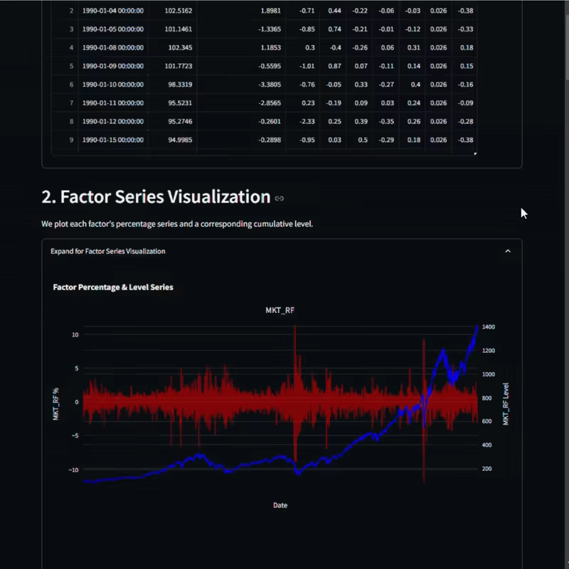
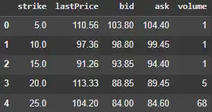
Figure 1. Raw option chain data before filtering. It shows strike prices, last traded prices, bid-ask quotes, and volume.

The data has a shape of (50, 5). However, many of these options are iliquid and will distort probability estimates. Only actively traded options are kept.

We define a function that removes options if:

  • Volume is too low (below a set threshold).
  • Bid price is zero (indicating no active buyers).
  • Bid-ask spread is too wide, meaning poor liquidity.
				
					# Function to filter out illiquid options
def filter_liquid_options(df, min_volume, max_spread_ratio):
    spread = df["ask"] - df["bid"]
    liquid_df = df[
        (df["volume"] >= min_volume) &
        (df["bid"] > 0) &
        ((spread := df["ask"] - df["bid"]) / df["ask"] <= max_spread_ratio)
    ]
    return liquid_df

# Apply filtering
filtered_calls_df = filter_liquid_options(calls_df, min_volume, max_spread_ratio)

# Display filtered data
filtered_calls_df.head()
				
			
Figure 2 Filtered option chain data after removing illiquid contracts. (OPTIMIZED)

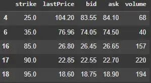
Figure 2. Filtered option chain data after removing illiquid contracts. It excludes options with low volume and wide bid-ask spreads.

The shape of the dataframe is now (25, 5). We continue the analysis with this dataframe.

3. Calculating Implied Volatility (IV)

As described, we calculate IV by inverting the Black-Scholes pricing model and solving for σ by numerically inverting this equation.

To find the IV that makes the Black-Scholes price match the observed market price, we use Brent’s method

Brent’s algorithm finds roots of a function in a given interval. Brent’s method is a smart way to find where a function equals zero. It combines two techniques:

  1. The Secant Method (Fast but Risky) — It estimates the answer by drawing a straight line between two points and seeing where it crosses zero. This works well when the function behaves nicely, but it can sometimes jump too far.
  2. The Bisection Method (Slow but Reliable) — It simply takes the middle point between two values and checks if the answer is there. This always works but takes more steps.

Brent’s method switches between these two approaches to get the best of both worlds — fast when possible, reliable when necessary.

Below, we calculate the IV and add it to the filtered_calls_df.

Prev Post

Finding Mispriced Stocks with a 6 Factor Model

post-bars
Mail Icon

Newsletter

Get Every Weekly Update & Insights

[mc4wp_form id=]

Leave a Comment