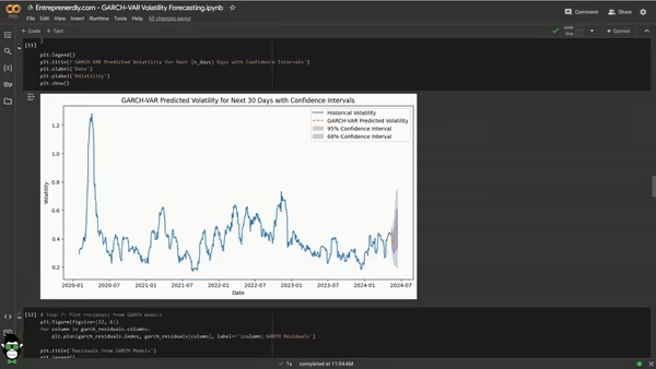
Volatility Predictions with External Variables and Confidence Intervals
Volatility forecasting is highly beneficial when pricing derivatives and or making risk management decisions. In this article, we apply a hybrid GARCH-VAR model specifically designed for forecasting rolling stock price volatility. Additionally, we incorporate external variables to improve the quality of the forecasts.
While traditional models often struggle with complex market dynamics, GARCH models handle time-varying volatility effectively. In contrast, VAR models capture the relationships between multiple variables across time. By combining these models, we aim to improve the accuracy of our volatility forecasts.
First, we preprocess the data by testing for stationarity and applying normalization techniques. After fitting the VAR model, we apply GARCH to the residuals to capture volatility clustering and refine the predictions by accounting for the time-varying volatility of the error terms. Next, we assess its performance by comparing forecasts with actuals, both in-sample and out-of-sample.
Our findings indicate that the hybrid model provides reliable volatility forecasts, especially accurate in estimating the future volatility direction. For those looking for a more advanced approach, Entreprenerdly offers a tool that leverages a stacked machine learning ensemble method with premium market data for forecasting volatility. You can find it here.
This Article is Structured as Follows:
- GARCH-VAR Model Background
- Gathering Data and Fitting the Model
- Model Forecasting and Confidence Intervals
- Predictions vs Actuals Assessment
1. The GARCH-VAR Model
The GARCH-VAR model brings together two important econometric models: Vector Autoregression (VAR) and Generalized Autoregressive Conditional Heteroskedasticity (GARCH).
With both we can capture (i) the relationships between multiple variables and (ii) the changing volatility that we often see in financial markets.
1.1 Vector Autoregression
VAR models handle multivariate time series data by capturing linear relationships among multiple variables. In a VAR model, each variable depends not only on its own past values but also on the past values of other variables in the system.
Therefore, VAR is particularly useful when trying to understand and forecast the dynamic interactions between several related time series, such as stock prices, economic indicators, or financial indices.
The mathematical representation of a VAR(p) model with k variables is:
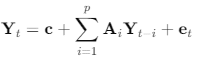
In the equation above:
- Yt is a k×1 vector of endogenous variables at time t.
- c is a k×1 vector of constants.
- Ai are k×k coefficient matrices for lag i.
- et is a k×1 vector of error terms.
In a VAR(1) model, for instance, each variable at time t depends on its own value and the values of the other variables from the previous period (lag 1). If we extend this to a VAR(p) model, each variable at time t would depend on its own and others’ values from the past p periods.
This framework is ideal for modeling financial data where variables often exhibit feedback relationships. For example, the price of a stock might depend on the prices of related stocks or market indices from previous periods, capturing potential interdependencies over time.
1.2 Generalized Autoregressive Conditional Heteroskedasticity
In contrast, GARCH models address volatility clustering in time series data. Volatility clustering refers to periods of high volatility followed by high volatility and periods of low volatility followed by low volatility. A GARCH(1,1) model captures this phenomenon by modeling the conditional variance of the error terms.
The model can be formally defined as
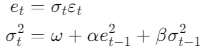
Where:
- et is the error term at time t.
- σt2 is the conditional variance at time t.
- εt is a white noise process with zero mean and unit variance.
- ω, α, and β are non-negative parameters with α+β<1 for stationarity.
The model states that the current variance σt2 depends on a constant ω, the squared error term from the previous period e2t−1, and the previous period’s variance σ2t−1.
“1,1” in GARCH(1,1) refers to the model using one lag for both the squared error term and the previous period’s variance when predicting the current variance.
Essentially, the model assumes that volatility today is influenced by both the size of the errors made in predicting the previous period and the volatility from the previous period.
1.3 Combining VAR and GARCH
The GARCH-VAR model allows us to capture both the mean dynamics with VAR and the volatility dynamics with GARCH. The process involves two main steps:
Estimate the VAR Model:
First, we estimate the VAR model to understand the linear relationships among the variables. This step identifies how variables influence each other over time. After fitting the VAR model, we obtain the residuals, which may show patterns of time-varying volatility.Model the Residuals with GARCH:
Second, we use GARCH models to handle the volatility in the residuals from the VAR model. With the GARCH model we capture the volatility clustering in the error terms—periods of high volatility followed by high volatility, and low volatility followed by low volatility.
The combined model can be expressed as:
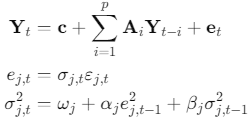
For j=1,2,…,k where k is the number of variables.
1.4 Forecasting with GARCH-VAR
To forecast future values and their variances, we follow these steps:
Forecast the Mean Using VAR
Use the estimated VAR model to forecast future values of Yt. This provides the expected mean values based on the linear relationships among variables.
Forecast the Variance Using GARCH
Use the GARCH models fitted to the residuals to forecast future variances σ2j,t. These forecasts capture the expected volatility in the error terms.
Adjust Forecasts with Variance Estimates
Combine the mean forecasts from the VAR model with the variance forecasts from the GARCH models. This accounts for both the expected value and the uncertainty due to volatility.
2. Data Preprocessing
Let’s start implementing the methodology. The first step is to gather the data we will be using in the forecasting process and transforming it in the necessary format for the GARCH-VAR model.
We will be using the libraries below. Key libraries include statsmodels for using the adfuller function for stationarity testing which tells us if we need to adjust our data. It also provides tools to implement the VAR. arch library will be used for fitting the GARCH model.
					# Import necessary libraries
import yfinance as yf
import numpy as np
import pandas as pd
from datetime import timedelta
from statsmodels.tsa.stattools import adfuller
from sklearn.preprocessing import MinMaxScaler
from statsmodels.tsa.api import VAR
from sklearn.metrics import mean_squared_error, mean_absolute_error
from arch import arch_model
import matplotlib.pyplot as plt
2.1 Data Collection
For this analysis, we focus on three main variables: stock prices (and volume), the S&P 500 Index, and the VIX Index. These variables have been selected due to their relevance and predictive power when forecasting stock price volatility.
The S&P 500 Index is commonly used in volatility forecasting models due to its ability to capture broader market movements. Andersen et al. (2003) highlight its predictive power for volatility when combined with individual stock data, showing that market-wide factors affect individual stock behavior. Additionally, Engle and Rangel (2008) discuss how incorporating indices like the S&P 500 improves model performance by accounting for market-wide shocks.
The VIX Index, a well-established measure of market volatility expectations, is known for its forward-looking properties. Giot (2005) demonstrates the significant role the VIX plays in predicting future stock volatility. Including the VIX enables us to capture not just historical volatility patterns but also the market’s expectations of future risk.
Please note that you may choose a different set of variables relevant to the stock in question, (e.g. semiconductor aggregates such as SOX Index, macroeconomic indicators like interest rates or inflation, or industry-specific factors such as global chip demand). With granger casuality you can assess wether these variables are relevant and improve the models.
					# Configuration section: Allows easy modification of tickers and settings
tickers = {
    'stock': 'ASML',  # Main stock ticker
    'sp500': '^GSPC',  # S&P 500 index
    'vix': '^VIX',     # VIX index
}
start_date = "2020-01-01"
end_date = "2024-05-15"
rolling_window = 21  # Rolling window for volatility
n_days = 30  # Number of future days to predict

# Downloading the data
data = {}
for name, ticker in tickers.items():
    data[name] = yf.download(ticker, start=start_date, end=end_date)
2.2 Data Preprocessing
We start by calculating log returns for the stock price and the S&P 500. Log returns focus on percentage changes, which normalizes the data and provides a more stable basis for modeling volatility. This avoids distortions caused by large price differences.
Next, we compute rolling volatility using a 21-day window. This approach tracks how volatility changes over time to provide a smoother view of market dynamics while focusing on short-term fluctuations. The 21-day window reflects a typical monthly trading patterns.
After processing each dataset, we merge the data for ASML, the S&P 500, and the VIX into a single DataFrame. This merged dataset includes:
- ASML volatility
- S&P 500 adjusted close prices
- S&P 500 volatility
- Log of VIX values
- S&P 500 returns
- ASML trading volume
- ASML returns
We drop any rows with missing values to ensure data integrity.
					# Calculate returns and volatility for the stock
data['stock']['Log_Returns'] = np.log(data['stock']['Adj Close'] / data['stock']['Adj Close'].shift(1))
data['stock']['Volatility'] = data['stock']['Log_Returns'].rolling(window=rolling_window).std() * np.sqrt(252)
data['stock'] = data['stock'].dropna()

# Calculate log returns and rolling volatility for SP500
data['sp500']['Log_Returns'] = np.log(data['sp500']['Adj Close'] / data['sp500']['Adj Close'].shift(1))
data['sp500']['SP500_Volatility'] = data['sp500']['Log_Returns'].rolling(window=rolling_window).std() * np.sqrt(252)
data['sp500'] = data['sp500'].dropna()

# Merge data into a single DataFrame
merged_data = data['stock'][['Volatility']].copy()
merged_data['SP500'] = data['sp500']['Adj Close']
merged_data['SP500_Volatility'] = data['sp500']['SP500_Volatility']
merged_data['VIX'] = np.log(data['vix']['Adj Close'])
merged_data['SP500_Returns'] = data['sp500']['Log_Returns']
merged_data['Volume'] = data['stock']['Volume']
merged_data['Stock_Returns'] = data['stock']['Log_Returns']

# Clean the merged data
merged_data = merged_data.dropna()
2.3 Stationarity Testing
Time series data often exhibit non-stationarity. For many Econometric models, data needs to be stationary. This means that its statistical properties like mean and variance should remain constant over time.
Non-stationary data can result in unreliable predictions, as models struggle with fluctuating trends. To check for stationarity, we use the Augmented Dickey-Fuller (ADF) test, which tests for a unit root. A p-value below 0.05 suggests the series is stationary, while a higher value indicates the presence of a unit root, requiring transformation.
If the data is non-stationary, we apply differencing, which involves subtracting the current value from the previous value to remove trends:
However, differencing can result in some loss of information. To mitigate this, other approaches may be considered such as Box-Cox Transformation.
The Box-Cox method stabilizes variance and makes the data more normal-like without directly differencing. This method can handle heteroscedasticity (non-constant variance) and is especially useful if standard differencing removes too much information.
					# ADF test for stationarity and automatic differencing
def check_stationarity_and_difference(df):
    for column in df.columns:
        result = adfuller(df[column].dropna())
        p_value = result[1]
        if p_value > 0.05:  # Non-stationary series
            df[column] = df[column].diff().dropna()

# Check for stationarity and apply differencing where necessary
merged_data_diff = merged_data.copy()
check_stationarity_and_difference(merged_data_diff)
merged_data_diff = merged_data_diff.dropna()
2.4 Data Normalization
We normalize the data using Min-Max scaling, which transforms all variables into a range between 0 and 1. This ensures that variables with different scales (like prices and returns) contribute equally to the model, preventing any one variable from dominating the analysis.
More articles worth reading:
Implied Volatility Analysis for Insights on Market Sentiment
Assessing Future Stock Price Movements With Historical & Implied Volatility

Newsletter