Who, What, and When: Transactional-Level Analysis of Senators' Trades with Accuracy Measuremenets and Trends Through the FMP API and the SEC website
Members of the U.S. Congress trade stocks, potentially leading to conflicts of interest. For those interested in Congress stock trades, tracking these transactions is crucial for transparency and spotting investment opportunities.
Given the mandatory public disclosure of their trades, an astute observer who knows how to track these trades could identify invesment opportunities.
This article shows how to examine in detail the individual trades of Senators, identifying specific asset class traded, the stock market symbol, the transaction date, and the approximate investment amount.
Furthermore, our primary data source will be the Financial Modeling Prep (FMP) API, which provides access to a comprehensive dataset of stock trades by members of the United States Senate.
Additionally, we will discuss the possibility of tracking these trades manually through the Securities and Exchange Commission (SEC) website, offering an open-source alternative.

We will cover various aspects of working with this data, including:
- Fetch and preprocess the vast amount of financial data, in this case the Senators’ Trades, via the FMP API
- Analyze transactions by type and asset, identify key senators and stocks, and assess trade signal accuracy
- Generate visualizations: transaction type bar charts, price trends with transactions, and senator summaries
- Automating tracking of Congressional trades using the SEC website with a Selenium
1. Understanding the Data Source
The Financial Modeling Prep (FMP) API provides programmatic access to a comprehensive financial data set, including historical Fundamental Data.
Notably, the FMP API serves as the primary resource for extracting detailed transaction information on Senators’ stock trades, crucial for those tracking Congress stock trades. You can sign up for the API here.
On the other hand, the Senate’s financial disclosure website serves as the direct source of public records, detailing the financial activities of Senators.
Moreover, it offers a more manual approach to data retrieval, allowing users to search and view disclosures on individual transactions. With some astuteness, this process can also be automated.
It’s important to note that this analysis concentrates on data pertaining to the Senate. The House of Representatives maintains a separate dataset with similar value for financial disclosure analysis. We will delve into this data source in a future article to provide a more holistic perspective on congressional trading activity.
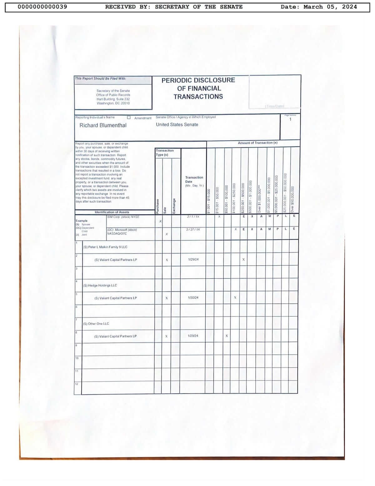
Figure. 1: Example of a Periodic Transaction Report by a Senator as filed with the Secretary of the Senate.
2. Analyzing Senate Trades with the FMP API
2.1 Retrieving the the dataset
We start by collecting data from the Financial Modeling Prep (FMP) API. This process involves fetching data across multiple pages to compile a comprehensive dataset of 3000 transactions and 13 columns of data.
FMP grants access to a wide array of financial data, including but not limited to, stock market transactions made by members of the United States Senate. Sign up for the API here.

The Python requests library facilitates this data retrieval, parsing JSON responses into a structured pandas DataFrame for analysis. For each page of the API response, we construct a request URL and send a GET request to the FMP API endpoint.
					import requests
import pandas as pd

def fetch_senate_trading_data(api_key, pages=30):
    all_data = []
    base_url = "https://financialmodelingprep.com/api/v4/senate-trading-rss-feed"

    for page in range(pages):
        url = f"{base_url}?page={page}&apikey={api_key}"
        response = requests.get(url)
        if response.status_code == 200:
            page_data = response.json()
            if page_data:
                all_data.extend(page_data)
            else:
                break  # Stop if a page has no data
        else:
            print(f"Failed to retrieve data for page {page}. Status code: {response.status_code}")
            break

    return pd.DataFrame(all_data)

# Use your API key here
api_key = ""
senate_trading_df = fetch_senate_trading_data(api_key, pages = 30)

# Optional: save the dataframe to a CSV file
# senate_trading_df.to_csv("senate_trading_data.csv", index=False)

senate_trading_df.head(10)

# Use this code if you'd like to download the data from gdrive to continue the analysis later on

'''
import requests

def download_file_from_google_drive(file_id, destination):
    URL = "https://drive.google.com/uc?export=download"

    session = requests.Session()

    response = session.get(URL, params = { 'id' : file_id }, stream = True)
    token = get_confirm_token(response)

    if token:
        params = { 'id' : file_id, 'confirm' : token }
        response = session.get(URL, params = params, stream = True)

    save_response_content(response, destination)

def get_confirm_token(response):
    for key, value in response.cookies.items():
        if key.startswith('download_warning'):
            return value

    return None

def save_response_content(response, destination):
    CHUNK_SIZE = 32768

    with open(destination, "wb") as f:
        for chunk in response.iter_content(CHUNK_SIZE):
            if chunk: # filter out keep-alive new chunks
                f.write(chunk)

# Use the file ID and specify the destination filename
file_id = '1znOQ7WGZt54c37o7qivIzwscqkRo-qYC'
destination = 'senate_trading_data.json' # Or any other path where you want to save the file

download_file_from_google_drive(file_id, destination)

senate_trading_df = pd.read_json('senate_trading_data.json', lines=True)

print(f"File has been downloaded and saved to {destination}.")

'''
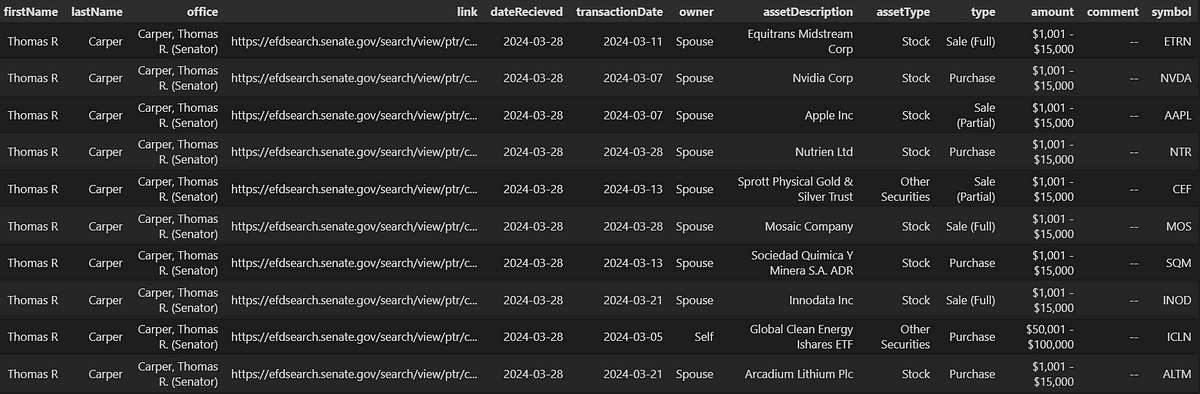
Figure. 2: Dataset extracted from the Financial Modeling Prep API showing individual stock market transactions by Senators.
2.2 Most Traded Asset Classes
With the Senate trading dataset in hand, our next objective is to explore the data to identify the asset classes that Senators are most inclined to trade.
This step shows the diversity of assets under consideration but also sheds light on Senators’ investment preferences and risk appetites.
Utilizing pandas, we segment the data based on two primary dimensions: the type of asset (e.g., stocks, bonds, crypto, etc) and the nature of the transaction (purchase, sale).
Analysis of the dataset reveals that stocks are the most frequently traded asset among Senators, highlighting their prominence in Congress stock trades.
					import matplotlib.pyplot as plt
import numpy as np
import pandas as pd

# Grouping and structuring the data for plotting
grouped_data = senate_trading_df.groupby(['assetType', 'type']).size().unstack(fill_value=0)

# Calculate a 'Total' transactions column for sorting purposes
grouped_data['Total'] = grouped_data.sum(axis=1)

# Sort the DataFrame by 'Total' transactions in descending order and drop the 'Total' column for plotting
grouped_data_sorted = grouped_data.sort_values(by='Total', ascending=False).drop(columns='Total')

# Now, plotting based on the sorted DataFrame
fig, ax = plt.subplots(figsize=(16, 8))

# Recalculate indices for the sorted DataFrame
ind = np.arange(len(grouped_data_sorted))

# Plotting Purchase, Sale (Full), and Sale (Partial) bars based on the sorted data
purchases = ax.bar(ind - width/2, grouped_data_sorted['Purchase'], width, label='Purchase', color='lightgreen')
sales_full = ax.bar(ind + width/2, grouped_data_sorted['Sale (Full)'], width, label='Sale (Full)', color='salmon')
sales_partial = ax.bar(ind + width/2, grouped_data_sorted['Sale (Partial)'], width, bottom=grouped_data_sorted['Sale (Full)'],
                       label='Sale (Partial)', color='darkred')

ax.set_xlabel('Asset Type', fontsize=14)
ax.set_ylabel('Frequency', fontsize=14)
ax.set_title('Transactions by Asset Type and Transaction Type (Sorted)', fontsize=16)
ax.set_xticks(ind)
ax.set_xticklabels(grouped_data_sorted.index, rotation=45)
ax.legend()

# Adjusting the annotate_bars function to work with sorted data
def annotate_bars(bars, offset=0):
    for bar in bars:
        height = bar.get_height()
        ax.annotate(f'{height}',
                    xy=(bar.get_x() + bar.get_width() / 2, height),
                    xytext=(0, offset),  # Offset to adjust the annotation position
                    textcoords="offset points",
                    ha='center', va='bottom')

# Annotating each category of bars
annotate_bars(purchases)
annotate_bars(sales_full, 3)
annotate_bars(sales_partial, 3)

plt.tight_layout()
plt.show()

Figure. 3: Senate Transactions by Asset Type and Transaction Type from 2019 to 2024.
2.3 Distribution of Most Traded Symbols
We progress the analysis by focusing on the distribution of the most actively traded symbols within the Senate’s transaction dataset.
This analysis aims to identify which stocks, bonds, or other financial instruments are favored by Senators and by how much.
- To achieve this, the dataset is first augmented to include a numeric representation of transaction amounts, transforming ranges into average values for each transaction.
- Subsequently, the dataset is grouped by symbol and transaction type, aggregating the count and sum of average transaction amounts. This step enables the identification of not only the most traded symbols but also the magnitude of transactions associated with each symbol.
- For visual representation, a composite bar chart is constructed, delineating the frequency of purchase and sale transactions across the top traded symbols. This chart provides a visual comparison between different securities.
					import matplotlib.pyplot as plt
import numpy as np
import pandas as pd
import re

# Function to parse and average amounts from the 'amount' column
def parse_amount_range(amount_range):
    numbers = [int(n.replace(',', '')) for n in re.findall(r'\b\d[\d,]*\b', amount_range)]
    return sum(numbers) / len(numbers) if numbers else 0

# Updated function to simplify amount for display, accommodating both thousands and millions
def simplify_amount(amount):
    """Converts an amount to a string with thousands ('k') or millions ('m') suffix, rounded to 1 decimal place."""
    if amount >= 1_000_000:
        return f'{amount/1_000_000:.1f}m'
    elif amount >= 1000:
        return f'{amount/1000:.1f}k'
    else:
        return str(amount)

# Define the number of top symbols you want to plot
top_n = 25

# Apply the parsing function to each amount and create a new 'avg_amount' column
senate_trading_df['avg_amount'] = senate_trading_df['amount'].apply(parse_amount_range)

# Group by 'symbol' and 'type', then aggregate
grouped_data = senate_trading_df.groupby(['symbol', 'type']).agg(count=('symbol', 'size'), sum_avg_amount=('avg_amount', 'sum')).unstack(fill_value=0)

# Simplify column names
grouped_data.columns = [' '.join(col).strip() for col in grouped_data.columns.values]

# Calculate a total transactions column for sorting
grouped_data['Total transactions'] = grouped_data.filter(like='count').sum(axis=1)

# Sort by total transactions in descending order and select top N symbols
grouped_data_sorted = grouped_data.sort_values('Total transactions', ascending=False).head(top_n)

# Plotting setup
fig, ax = plt.subplots(figsize=(20, 10))
ind = np.arange(len(grouped_data_sorted))  # X locations
width = 0.25  # Bar width

# Plotting bars
types = ['Purchase', 'Sale (Full)', 'Sale (Partial)']
colors = ['lightgreen', 'salmon', 'darkred']

for i, transaction_type in enumerate(types):
    counts = grouped_data_sorted[f'count {transaction_type}']
    ax.bar(ind + i * width, counts, width, label=transaction_type, color=colors[i])

    # Annotation for counts
    for j, val in enumerate(counts):
        ax.text(j + i * width, val + 0.01 * max(counts), f'{val}', ha='center', va='bottom')

# Adjusted to annotate the sum of avg_amounts instead of the average
for i, transaction_type in enumerate(types):
    sum_avg_amounts = grouped_data_sorted[f'sum_avg_amount {transaction_type}']
    for j, val in enumerate(sum_avg_amounts):
        simplified_amount = simplify_amount(val)  # Use the updated function here
        count = grouped_data_sorted[f'count {transaction_type}'].iloc[j]
        if count > 0:  # Only annotate if count > 0
            # Positioning slightly above the count annotation, with adjustments for sum
            vertical_position = count + 0.05 * max(counts)
            ax.text(j + i * width, vertical_position, f'${simplified_amount}', ha='center', va='bottom', fontsize=9, color='blue', rotation=90)

ax.set_xlabel('Symbol')
ax.set_ylabel('Transactions Count')
ax.set_title(f"Top {top_n} Symbols by Transaction Count and Type with labels for Average Total Amount ({senate_trading_df['transactionDate'].min()} to {senate_trading_df['transactionDate'].max()})")

ax.set_xticks(ind + width)
ax.set_xticklabels(grouped_data_sorted.index, rotation=45)
ax.legend()

plt.tight_layout()
plt.show()

Figure. 4: Analysis of the Top 25 Most Traded Stock Symbols in the Senate, Highlighting Transaction Counts and Total Average Amounts invested from 2019 to 2024.
2.4 Buy and Sell Signals Across Time
We now examine the temporal dynamics of buy and sell signals within the Senate trading data, focusing on their alignment with market movements. Moreover, by overlaying transaction data onto stock price timelines, we aim to assess the timing and potential foresight of these Congress stock trades.
Utilizing yfinance for stock data retrieval and matplotlib for visualization, we plot the closing prices of stocks over time, annotating buy and sell transactions. This visual approach allows for an immediate understanding of how Senate trades are positioned relative to market trends.
Beyond mere visualization, we extend the analysis to quantitatively assess the accuracy of these transactions. This involves calculating the percentage change in stock prices following a transaction, within a defined window (e.g., 30 days).
					import yfinance as yf
import matplotlib.pyplot as plt
import pandas as pd
import numpy as np
from matplotlib.lines import Line2D
import matplotlib.dates as mdates  # Import for handling date formatting

# Parameters
t_days = 30  # Number of days to check for accuracy
transaction_amount_threshold = 10000  # Amount threshold for visualization
top_n_symbols = 5

# Assuming 'senate_trading_df' is already defined
senate_trading_df['transactionDate'] = pd.to_datetime(senate_trading_df['transactionDate'])

def amount_to_numeric(amount_str):
    amounts = [int(s.replace(',', '').replace('$', '')) for s in amount_str.split('-')]
    return sum(amounts) / len(amounts)

senate_trading_df['numeric_amount'] = senate_trading_df['amount'].apply(amount_to_numeric)
senate_trading_df['transactionType'] = np.where(senate_trading_df['type'].str.contains('Purchase'), 'Buy', 'Sell')
total_avg_amount_by_date_and_type = senate_trading_df.groupby(['transactionDate', 'symbol', 'transactionType']).agg({'numeric_amount': 'sum'}).reset_index()

start_date = senate_trading_df['transactionDate'].min()
end_date = senate_trading_df['transactionDate'].max() + pd.Timedelta(days=5)  # Extend for accuracy check

top_symbols = senate_trading_df['symbol'].value_counts().head(top_n_symbols).index.tolist()

fig, axes = plt.subplots(nrows=len(top_symbols), figsize=(16, 4 * len(top_symbols)), squeeze=False)

#accuracies = []

for i, symbol in enumerate(top_symbols):
    ax = axes[i][0]
    stock_data = yf.download(symbol, start=start_date, end=end_date)

    ax.plot(stock_data.index, stock_data['Close'], label=f'{symbol} Close Price', color='blue')

    ax2 = ax.twinx()
    ax2.fill_between(stock_data.index, 0, stock_data['Volume'], color='grey', alpha=0.3)
    ax2.set_ylabel('Volume', color='grey')
    ax2.tick_params(axis='y', labelcolor='grey')
    ax2.set_ylim(0, max(stock_data['Volume'])*4)

    correct_buy_signals, total_buy_signals = 0, 0
    correct_sell_signals, total_sell_signals = 0, 0

    symbol_transactions = total_avg_amount_by_date_and_type[
        (total_avg_amount_by_date_and_type['symbol'] == symbol) &
        (total_avg_amount_by_date_and_type['numeric_amount'] > transaction_amount_threshold)]

    for _, row in symbol_transactions.iterrows():
        transaction_date = row['transactionDate']
        if transaction_date in stock_data.index:
            color = 'green' if row['transactionType'] == 'Buy' else 'red'
            price_on_transaction = stock_data.at[transaction_date, 'Close']

            # Scaling marker size based on transaction amount
            # ax.scatter(transaction_date, price_on_transaction, s=np.log(row['numeric_amount'] + 1) * 10, color=color, alpha=0.5) # log scaling
            # ax.scatter(transaction_date, price_on_transaction, s=row['numeric_amount'] / 1000 * 10, color=color, alpha=0.5) # linear scaling
            ax.scatter(transaction_date, price_on_transaction, s=np.sqrt(row['numeric_amount']) * 5, color=color, alpha=0.5) # square root scaling

            ax.axvline(x=transaction_date, color=color, linestyle='--', alpha=0.5)

            try:
                price_after_t_days = stock_data.loc[transaction_date + pd.Timedelta(days=t_days), 'Close']
                signal_correct = (row['transactionType'] == 'Buy' and price_after_t_days > price_on_transaction) or \
                                 (row['transactionType'] == 'Sell' and price_after_t_days < price_on_transaction)

                if row['transactionType'] == 'Buy':
                    total_buy_signals += 1
                    if signal_correct:
                        correct_buy_signals += 1
                elif row['transactionType'] == 'Sell':
                    total_sell_signals += 1
                    if signal_correct:
                        correct_sell_signals += 1
            except KeyError:
                # Skip if no price data available for the date after t_days
                continue

    buy_accuracy = (correct_buy_signals / total_buy_signals) * 100 if total_buy_signals > 0 else 0
    sell_accuracy = (correct_sell_signals / total_sell_signals) * 100 if total_sell_signals > 0 else 0

    # Collect accuracies for each symbol for further analysis or display
    #accuracies.append({'symbol': symbol, 'buy_accuracy': buy_accuracy, 'sell_accuracy': sell_accuracy})

    ax.set_title(f'{symbol} - Senate Trades - Buy Accuracy: {buy_accuracy:.2f}%, Sell Accuracy: {sell_accuracy:.2f}% - Transactions over {transaction_amount_threshold}$')
    ax.set_xlabel('Date')
    ax.set_ylabel('Price')

    ax.legend(handles=[Line2D([0], [0], color='blue', lw=2, label=f'{symbol} Close Price'),
                       Line2D([0], [0], marker='o', color='w', markerfacecolor='green', markersize=10, label='Buy Signal (Marker Size Proportional to Amount)'),
                       Line2D([0], [0], marker='o', color='w', markerfacecolor='red', markersize=10, label='Sell Signal (Marker Size Proportional to Amount)')],
              loc='upper left')

    ax.xaxis.set_major_locator(mdates.MonthLocator())
    ax.xaxis.set_major_formatter(mdates.DateFormatter('%Y-%m'))
    plt.setp(ax.xaxis.get_majorticklabels(), rotation=45)

plt.tight_layout()
plt.show()

# Optional: Print or analyze collected accuracies
# print(accuracies)
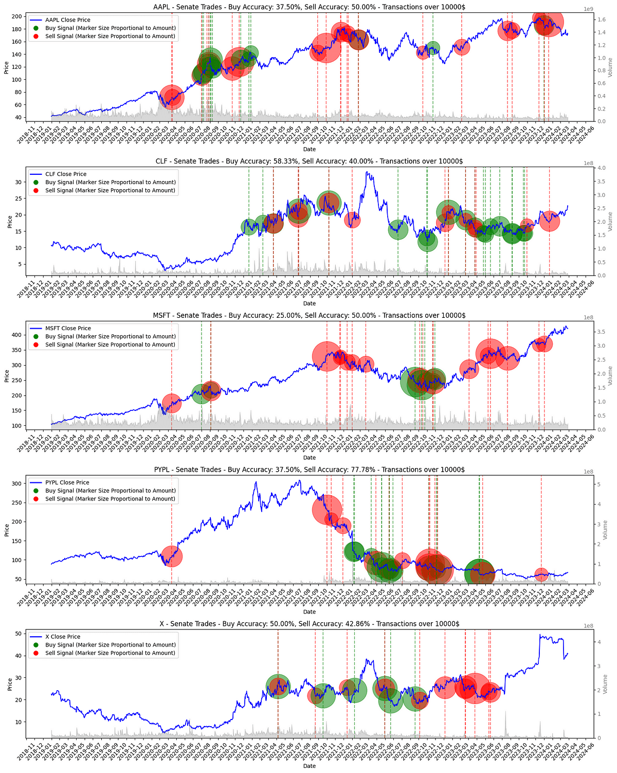
Figure. 5: Top 5 Most traded stocks: showing stock price trends and transaction points by overlaying Senate buy and sell transactions on stock performance, indicating potential predictive signals.
2.5 Trading Accuracy Across Senators
This section aims to quantify the trading performance of Senators by analyzing the accuracy of their buy and sell transactions over a specified period. By correlating these transactions with subsequent market movements, we establish a metric for evaluating the foresight and financial acumen of individual Senators.
					import pandas as pd
import yfinance as yf
from datetime import timedelta

n_days = 30  # Days after the transaction to calculate accuracy
top_n_senators = 25
top_n_symbols = 5

# Combine names, convert dates, and convert amounts
senate_trading_df['Senator'] = senate_trading_df['firstName'] + " " + senate_trading_df['lastName']
senate_trading_df['transactionDate'] = pd.to_datetime(senate_trading_df['transactionDate'])
senate_trading_df['amountNumeric'] = senate_trading_df['amount'].apply(
    lambda x: pd.to_numeric(x.split(' - ')[0].replace('$', '').replace(',', '')))

# Determine the top 2 senators and their symbols
top_senators = senate_trading_df['Senator'].value_counts().nlargest(top_n_senators).index.tolist()
top_symbols_per_senator = {
    senator: senate_trading_df[senate_trading_df['Senator'] == senator]['symbol'].value_counts().nlargest(top_n_symbols).index.tolist()
    for senator in top_senators
}

# Fetch data for unique symbols
unique_symbols = set([symbol for symbols in top_symbols_per_senator.values() for symbol in symbols])
symbol_data = {}
for symbol in unique_symbols:
    try:
        min_date = senate_trading_df[senate_trading_df['symbol'] == symbol]['transactionDate'].min()
        max_date = senate_trading_df[senate_trading_df['symbol'] == symbol]['transactionDate'].max() + timedelta(days=n_days)
        data = yf.download(symbol, start=min_date.strftime('%Y-%m-%d'), end=max_date.strftime('%Y-%m-%d'))
        if not data.empty:
            symbol_data[symbol] = data
        else:
            print(f"No data found for {symbol}")
    except Exception as e:
        print(f"Error downloading data for {symbol}: {e}")

# Calculate accuracies for top senators
results = []
for senator, symbols in top_symbols_per_senator.items():
    # Initialize lists to store accuracies for buy and sell transactions
    buy_accuracies, sell_accuracies = [], []

    for symbol in symbols:
        transactions = senate_trading_df[(senate_trading_df['Senator'] == senator) & (senate_trading_df['symbol'] == symbol)]
        for _, transaction in transactions.iterrows():
            try:
                # Ensure we have pre-fetched data for this symbol
                if symbol in symbol_data:
                    data = symbol_data[symbol]
                    # Find relevant prices for the transaction date
                    open_price = data.loc[data.index >= transaction['transactionDate']]['Open'].iloc[0]
                    close_price = data.loc[data.index <= transaction['transactionDate'] + timedelta(days=n_days)]['Close'].iloc[-1]
                    accuracy = (close_price - open_price) / open_price

                    # Append accuracy based on the type of transaction
                    if transaction['type'] == 'Purchase':
                        buy_accuracies.append(accuracy)
                    else:  # Sale
                        sell_accuracies.append(accuracy)
            except Exception as e:
                print(f"Error processing transaction for {symbol} on {transaction['transactionDate']}: {e}")

    # Compile the results for this senator
    avg_buy_accuracy = sum(buy_accuracies) / len(buy_accuracies) if buy_accuracies else 0
    avg_sell_accuracy = sum(sell_accuracies) / len(sell_accuracies) if sell_accuracies else 0
    avg_transaction_amount = transactions['amountNumeric'].mean()
    total_transactions = transactions.shape[0]

    results.append({
        'Senator': senator,
        'Average Buy Accuracy': avg_buy_accuracy,
        'Average Sell Accuracy': avg_sell_accuracy,
        'Average Transaction Amount': avg_transaction_amount,
        'Total Transactions': total_transactions,
        'Top n symbols': ', '.join(symbols)
    })

# Convert the results into a DataFrame
final_df = pd.DataFrame(results)

# Optionally, sort the DataFrame as needed
final_df = final_df.sort_values(by=['Total Transactions', 'Average Transaction Amount'], ascending=False)

final_df

Figure. 6: A tabular summary quantifying the trading accuracy of top Senators and their most traded stocks, measured over a set period.
3. Automating Manual Retrieval Process
Automating the retrieval of Senate stock trades involves three key steps: 1) navigating to and searching the Senate’s financial disclosure website, 2) collecting links to individual reports, and finally 3) scraping the content of these reports. Below, we detail each step utilizing Selenium, a tool for automating web browsers.
3.1 Agreement Acceptance and Performing Search
Navigating to the Senate’s financial disclosure website requires initially accepting a mandatory agreement that governs the lawful use of disclosed information, as per the Ethics in Government Act of 1978.
To automate this process, we employ Selenium scripts to mimic user actions and accept the agreement by identifying and clicking the requisite checkbox. Post-acceptance, Selenium handles a short pause to accommodate the website’s processing time before proceeding to the main search page.
Subsequently, the script is set up to target the retrieval of Congress stock trades, configuring search filters to extract “Periodic Transaction Reports” within a chosen date range. Focusing on these transactions allows for a targeted analysis of Senators’ trading activities, filtering out irrelevant data:

Newsletter