Experience the Future of Intelligent Investing Today
Back To Top
Experience the Future of Intelligent Investing Today
You know, when you look at how stocks move up and down, it can seem as unpredictable as ocean waves. However, just like scientists can predict wave movements by understanding the underlying currents, we can also try to make sense of stock market patterns using similar tools – like the wavelet transform.
First off, by utilizing the wavelet transform, we’re essentially peering beneath the surface to uncover the deep currents driving stock prices. Furthermore, this isn’t merely about crunching numbers and data. We’re taking the seemingly erratic stock behaviors and attempting to find some rhythm behind it all.

At the very core, a wavelet is like a brief vibration or oscillation that packs all its energy into a short burst of time. It’s intense but fades out quickly. For example, think about striking a drum – that sound is powerful but doesn’t last very long.
Now, this short-lived nature of wavelets is actually really useful when analyzing financial data that keeps changing over time. The statistical properties aren’t constant, they fluctuate. And wavelets can handle that.
Using a wavelet transform is kind of like getting a microscope to examine stock data up close. With it, you can see the big overall trends, but also zoom in on those tiny, minute fluctuations. It lets you view the details from multiple perspectives.
Many might think, why not just use the Fourier Transform, which is a very popular tool to analyze signals? Fourier Transform breaks down a signal into its constituent sinusoids. However, its Achilles’ heel is its inability to provide both time and frequency information simultaneously.
While it can tell us the frequencies present, it’s often oblivious to when they occur. Unlike its Fourier counterpart, Wavelet Transform captures both the frequency and the time, providing a time-frequency representation of the signal.
Mathematically, the Wavelet Transform can be represented as:

Equation. 1: Wavelet Transform Representation
Where:
In essence, we’re moving our wavelet ψ across the stock data f(t), looking for places where they align well. This gives us the wavelet coefficients W(b) which tell us how strongly the stock data matches the wavelet at each point in time. Put simply, the better the match at any given point, the higher the value of W.


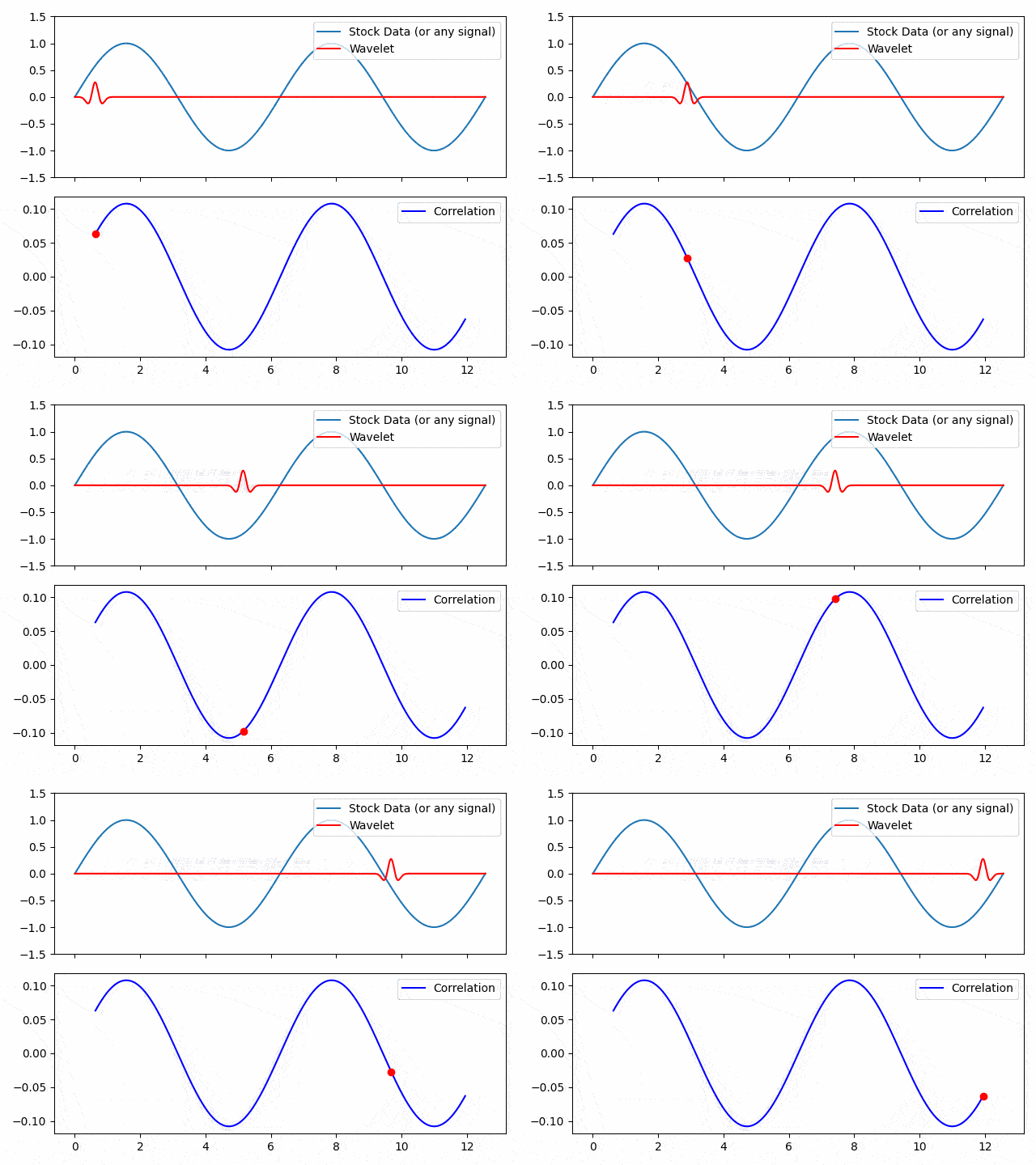
Figure. 1: On the left, the Continuous Wavelet Transform (CWT) visualizes stock data at different scales, capturing varied time durations. On the right, a Ricker wavelet moves through the stock signal, with its correlation shown below. Together, they spotlight how wavelets localize patterns in stock data, distinguishing short-term fluctuations from long-term trends.
In the presented visualizations, we see the mechanism of the Wavelet Transform as applied to time series data, such as stock prices. On the left, we see a vivid portrayal of the Continuous Wavelet Transform (CWT) applied to stock data. Each frame of the animation displays wavelet coefficients at a different scale, capturing patterns that exist at varying time durations. Wider wavelets detect longer-term trends, while narrower ones focus on short-term fluctuations.
Beside it, on the right, is a depiction of how a wavelet, in this case, a Ricker wavelet, traverses through the stock signal. As the wavelet slides across, it gets multiplied point-by-point with the stock data, and the resultant values are summed up to produce a single coefficient. This ‘correlation’ is plotted below, with the red dot marking the current coefficient value as the wavelet moves. High peaks in the correlation plot indicate locations where the wavelet aligns well with the stock data, capturing specific patterns. In essence, this process is a systematic approach to unearth local patterns within vast time series data, offering a granular perspective that Fourier Transform might miss.
We’ll now delve into the Python implementation of the Wavelet Transform for deriving buy/sell signals from stock data which is what might be of interest to traders and Data Scientist. The code employs the Continuous Wavelet Transform to extract features that can indicate potential buy or sell moments in the stock’s historical data.
Ensure you have the required Python libraries. If not, they can be installed via pip:
pip install numpy pandas matplotlib yfinance scipy
Using the yfinance library, we can easily fetch stock data for analysis:
					import yfinance as yf

ticker = "SIE.DE"
stock_data = yf.download(ticker, start="2018-01-01", end="2023-12-30")
The scipy library provides the required functions to compute the CWT using the Ricker wavelet:
					from scipy import signal

widths = np.arange(1, 15)
cwt_result = signal.cwt(stock_data['Close'].values, signal.ricker, widths)
From the computed CWT, positive and negative coefficients can be extracted, indicating upward and downward movements in stock price, respectively.
					cwt_positive = np.where(cwt_result > 0, cwt_result, 0)
cwt_negative = np.where(cwt_result < 0, cwt_result, 0)

buy_signal = pd.Series(np.sum(cwt_positive, axis=0), index=stock_data.index)
sell_signal = pd.Series(-np.sum(cwt_negative, axis=0), index=stock_data.index)
Crossovers between buy and sell signals can potentially indicate trading opportunities.
					cross_above = (buy_signal >= sell_signal) & (buy_signal.shift(1) < sell_signal.shift(1))
cross_below = (buy_signal <= sell_signal) & (buy_signal.shift(1) > sell_signal.shift(1))
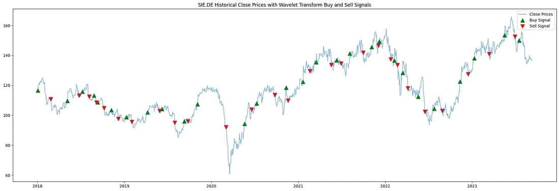
A visual representation can provide a clearer perspective on the buy/sell moments against the stock’s historical data:
					import matplotlib.pyplot as plt

plt.figure(figsize=(30, 6))
plt.plot(stock_data.index, stock_data['Close'], label='Close Prices', alpha=0.5)
plt.scatter(stock_data.index[cross_above], stock_data['Close'][cross_above], label='Buy Signal', marker='^', color='g')
plt.scatter(stock_data.index[cross_below], stock_data['Close'][cross_below], label='Sell Signal', marker='v', color='r')
plt.title(f'{ticker} Historical Close Prices with Wavelet Transform Buy and Sell Signals')
plt.legend()
plt.show()
Putting all the code together we get

Newsletter