Back To Top

August 20, 2024

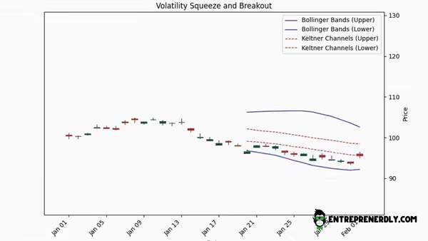
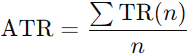
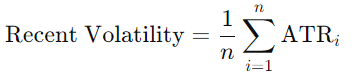
Identifying a Volatility Squeeze Algorithmically

Signal Generation Using Bollinger Bands and Keltner Channels

As a trader, one of the patterns to look for is a volatility squeeze. This occurs when market volatility tightens, often shown by the Bollinger Bands and Keltner Channels narrowing. Such a squeeze usually hints at a potential breakout.

By spotting these squeezes early, traders can position themselves ahead of significant market moves. This guide will dive into identifying volatility squeezes using algorithmic methods.

We’ll cover how to fine-tune the Bollinger Bands and Keltner Channels using walk-forward optimization. Plus, you’ll get full Python code to apply these techniques yourself.

volatility squeeze breakout example AVIF
This article is structured as follows:
  • Understanding Volatility Squeezes
  • Algorithmic Implementation
    • Key Indicator Functions
    • Walk-foward Optimization Routine
    • Identifying a Volatility Squeeze
  • Generating Buy and Sell Signals
  • Limitations and Improvements

1.Volatility Squeezes

A volatility squeeze happens when market volatility drops significantly, leading to a period of low volatility. This phase often sets the stage for a big price movement.

The concept is rooted in the idea that the market naturally cycles between high and low volatility. During low volatility, prices often consolidate, building up energy for a sharp move later.

How Traders Trade Volatility Squeeze

The typical approach to trading a volatility squeeze involves spotting the squeeze, confirming the breakout direction, and managing the trade with clear entry and exit strategies.

Identifying the Squeeze

Bollinger Bands and Keltner Channels are used to spot a squeeze. When Bollinger Bands narrow within the Keltner Channels, this is a sqeeze. This signals market consolidation. This is the calm before a potential breakout.

Entry Signals

Once a squeeze is detected, look for a breakout to determine the trade direction.

  • Buy Signal: A long position is triggered if the price breaks above both the upper Bollinger Band and the Keltner Channel.
  • Sell Signal: A short position is considered if the price drops below both the lower Bollinger Band and the Keltner Channel.

Volume is a critical confirmation tool here. An increase in volume during the breakout strengthens the signal, indicating that the move is backed by strong market participation.

Managing the Trade

After entering a trade based on the breakout, managing risk is essential. Traders use stop losses and set profit targets:

  • Stop Loss Placement: For long positions, place the stop loss just below the lower Bollinger Band. For short positions, place it just above the upper band. Alternatively, some traders use the ATR to set stop losses, positioning them a multiple of the ATR away from the entry point.

  • Profit Targets: These can be set at key levels, like the next Bollinger Band or based on a predefined risk-reward ratio, for instance often 1:2 or 1:3.

2. Bollinger Bands and Keltner Channels

2.1 Bollinger Bands

Bollinger Bands, developed by John Bollinger in the 1980s, are a volatility-based indicator that includes a moving average and two standard deviation lines plotted above and below this average. The upper and lower bands are calculated as:

formula Upper Bollinger Band
formula Lower Bollinger Band

SMA(n) is the simple moving average over periods. is the standard deviation of the price over periods. is the number of standard deviations (typically 2).

2.2 Keltner Channels

Keltner Channels are similar to Bollinger Bands but use the Average True Range instead of standard deviation to set the bands. The Keltner Channel consists of a moving average, usually an exponential moving average, with upper and lower bands calculated as:

formula 3. Upper Keltner Channel
formula 4 Lower Keltner Channel

EMA(n) is the exponential moving average over periods. ATR(n) is the average true range over periods.  is the ATR multiplier (commonly set to 1.5).

2.3 Average True Range (ATR)

ATR, developed by J. Welles Wilder, is a key volatility indicator. It measures the range of price movement over a period, including any gaps. The True Range (TR) for a single period is calculated as the maximum of the following:

  • Current High – Current Low: This gives the basic range for the period.
  • Absolute Value of Current High – Previous Close: Accounts for any upward gap from the previous close.
  • Absolute Value of Current Low – Previous Close: Accounts for any downward gap from the previous close.

The ATR is then determined as a moving average of the TR values over a specified number of periods :

formula 6 TR Formula

ATR provides a smoothed measure of volatility. This makes Keltner Channels responsive to price changes and providing a more stable measure of volatility compared to just standard deviation.

3. Algorithmic Implementation

To identify a volatility squeeze, we need to set up the right data and indicators. We start by pulling stock prices using yfinance, then use pandas to clean and organize the data.

Key indicators like Bollinger Bands and Keltner Channels are calculated to spot potential squeezes. The goal is to optimize the detection parameters for accuracy and also use confirmation indicators.

3.1 Libraries and Data

This function below gets us the asset price data we need. It’s rather straightfoward.

				
					import yfinance as yf
import numpy as np
import pandas as pd
import matplotlib.pyplot as plt
from itertools import product
import warnings
warnings.filterwarnings("ignore")  # Suppress warnings to keep the output clean

# Fetch data from yfinance
def get_stock_data(ticker, start_date, end_date):
    # Using yfinance to access historical stock data, ensuring we have the required price information for calculations.
    stock_data = yf.download(ticker, start=start_date, end=end_date)
    return stock_data


3.2 Key Indicator Functions

We use Bollinger Bands, Keltner Channels, and confirmation indicators like RSI and MACD to identify volatility squeezes. We use these indicators to validate whether a detected squeeze is likely to lead to a significant market move.

Bollinger Bands


# Calculate Bollinger Bands
def bollinger_bands(data, window=20, no_of_std=2):
    # Rolling mean and standard deviation provide a dynamic range to assess price volatility.
    rolling_mean = data['Close'].rolling(window).mean()
    rolling_std = data['Close'].rolling(window).std()

    # Bollinger Bands are calculated to identify periods of high or low volatility.
    data['Bollinger_High'] = rolling_mean + (rolling_std * no_of_std)
    data['Bollinger_Low'] = rolling_mean - (rolling_std * no_of_std)
    return data


Keltner Channels

				
					# Calculate Keltner Channels (Simplified without dynamic ATR multiplier)
def keltner_channel(data, window=20, atr_mult=1.5):
    # The True Range calculation is key to understanding the volatility by considering price gaps.
    data['Previous_Close'] = data['Close'].shift(1)
    data['TR'] = data[['High', 'Low', 'Previous_Close']].apply(lambda x: max(x[0] - x[1],
                                                                            abs(x[0] - x[2]),
                                                                            abs(x[1] - x[2])), axis=1)
    # ATR provides a smoothed measure of volatility, which is crucial for calculating the Keltner Channel.
    data['ATR'] = data['TR'].rolling(window).mean()

    # Keltner Channels use ATR to define the channel width around the moving average.
    rolling_mean = data['Close'].rolling(window).mean()
    data['Keltner_High'] = rolling_mean + (data['ATR'] * atr_mult)
    data['Keltner_Low'] = rolling_mean - (data['ATR'] * atr_mult)
    return data


Moving Average Filter

				
					# Add a moving average filter
def moving_average_filter(data, window=50):
    # A longer moving average helps smooth out price action, making it easier to identify trends and potential reversal points.
    data['MA'] = data['Close'].rolling(window=window).mean()
    return data

# Simplified confirmation indicators: RSI and MACD only
def add_confirmation_indicators(data, rsi_window=14, macd_short=12, macd_long=26, macd_signal=9):
    # RSI is used to measure momentum, giving us an idea of whether the stock is overbought or oversold.
    data['RSI'] = 100 - (100 / (1 + data['Close'].diff(1).clip(lower=0).rolling(window=rsi_window).mean() /
                                  -data['Close'].diff(1).clip(upper=0).rolling(window=rsi_window).mean()))

    # MACD and its signal line are calculated to assess the strength and direction of the trend.
    data['MACD'] = data['Close'].ewm(span=macd_short, adjust=False).mean() - data['Close'].ewm(span=macd_long, adjust=False).mean()
    data['MACD_Signal'] = data['MACD'].ewm(span=macd_signal, adjust=False).mean()

    return data


3.3 Identify Volatility Squeeze Parameters

To make the squeeze detection more reliable, we need to optimize these parameters dynamically, adjusting them based on the current market conditions. This approach helps us ensure that our squeeze detection adapts as volatility changes.

3.3.1 Volatility Squeeze Function

The process involves calculating a dynamic squeeze threshold based on the stock’s ATR

Here’s how it works:

1. Calculate Recent Volatility: We start by computing the rolling mean of the ATR over a specified window. This gives us a sense of the recent volatility.

formula 7 Recent-Volatility

2. Dynamic Squeeze Threshold: Next, we adjust the base threshold using the recent volatility. The formula for the dynamic squeeze threshold is:

formula 8 Dynamic Sqeeze Threshold

This ensures that the threshold is higher in more volatile markets and lower when the market is calmer.

3. Identifying the Squeeze: A squeeze is identified when the Bollinger Bands fall within the Keltner Channels. We further filter these squeezes by checking the RSI and MACD to ensure that the conditions are favorable for a potential breakout.

4. Final Squeeze Signal: If all the conditions are met—meaning the Bollinger Bands are within the Keltner Channels, and the RSI and MACD indicators align—the squeeze indicator is set to 1.

More articles worth reading:

Implied Volatility Analysis for Insights on Market Sentiment

Dynamic Stop-Losses with Bayesian Walk-Forward Optimization

Prev Post

Earn $491 a day with $29,260 Bitmain Antminer AL1

Next Post

Calculate The Fair Value of Stocks Using DCF with Public…

post-bars
Mail Icon

Newsletter

Get Every Weekly Update & Insights

[mc4wp_form id=]

Leave a Comment