Not All Factors Are Created Equal - How to Find, Validate, and Test the Best Alpha Factors Using Alphalens in Python
Finding consistent alpha in the market is hard. Traders could rely on intuition, but this might not offer a systematic and clear edge.
The key is identifying repeatable and testable patterns — factors — that are correlated with future returns.
In this article, we will walk through a quantitative framework for evaluating the performance of alpha factors.
Using a simple mean-reversion strategy, we’ll compute Z-score factors across multiple stocks to identify key price deviations.
Factors will be analyzed in a cross-sectional manner using Alphalens. Stocks are then ranked into quantiles based on the strength of the factors
This article is structured as follows
- Constructing Simple Mean-Reversion Z-Score Factor
- Preparing a Factor Dataset for Alphalens
- Evaluating Factor Performance with Alphalens
- Key Limitations and Concluding Thoughts
End-to-end notebook is provided below so that you can adjust the parameters and strategy as needed.
1. Factor Investing and Alpha Generation
What Are Factors?
Factor investing is a systematic approach to selecting stocks based on quantifiable characteristics that explain differences in returns.
This concept dates back to Fama and French (1992), who introduced the Three-Factor Model, which expanded on the traditional Capital Asset Pricing Model by adding size and value factors to explain stock returns better.
Over time, researchers and practitioners have identified several other factors, including:
- Value: Stocks that appear cheap based on fundamentals (e.g., low P/E or P/B ratios) tend to outperform expensive stocks. (Fama & French, 1992)
- Momentum: Stocks that have performed well recently tend to continue performing well in the short term. (Jegadeesh & Titman, 1993)
- Quality: Stocks with strong profitability, low debt, and stable earnings deliver higher risk-adjusted returns. (Novy-Marx, 2013)
- Volatility & Low Beta: Lower-volatility stocks tend to produce better risk-adjusted returns than high-volatility stocks. (Baker, Bradley, & Wurgler, 2011)
- Formulaic Alphas: hand-crafted, rule-based trading signals derived from mathematical expressions applied to high-frequency price and volume data. (Zura Kakushadze, 2016)
Cross-Sectional Factor Analysis
Instead of analyzing a single stock, we evaluate a large set of stocks at each point in time. This is known as cross-sectional analysis, and it is widely used in quantitative finance to rank stocks based on factor strength.
For instance, we can rank all S&P 500 stocks by their Z-score and divide them into five quantiles:
- Top 20% (Q5): Stocks with the highest Z-scores (potential short candidates).
- Bottom 20% (Q1): Stocks with the lowest Z-scores (potential long candidates).
By tracking the performance of these quantiles over time, we can assess whether the factor is predictive. If Q1 consistently outperforms Q5, then the Z-score factor has value.
2. Constructing a Mean-Reversion Z-Score Factor
We implement a simple mean-reversion trading strategy to illustrate the construction of predictive factors.
Mean reversion is a well-studied short-term factor, rooted in behavioral finance — traders overreact to news, pushing prices away from their fair value, which leads to corrections.
To quantify these deviations, we compute a Z-score to measure the deviation of the current price from a long-term average.
EWMA-Based Z-Score Formula
For the long-term average estimation we use ‘Exponentially Weighted Moving Average’.
The Z-score in our implementation is calculated as:
where:
- Rt = log return at time t
- EWMAμ = exponentially weighted moving average of returns
- EWMAσ = exponentially weighted standard deviation of returns
To determine the optimal lookback period, we use a half-life parameter, which controls how quickly past data loses relevance.
A smaller half-life reacts faster to price changes, while a larger half-life smooths fluctuations more gradually.
Finally, we apply winsorization to remove extreme outliers, ensuring that rare price spikes or crashes do not distort the factor signal / quantiles.
					import numpy as np
import pandas as pd
import yfinance as yf
import matplotlib.pyplot as plt
import warnings
from scipy.stats.mstats import winsorize

warnings.filterwarnings("ignore")  # Suppress warnings for cleaner output
plt.style.use("dark_background")
					def compute_zscore(returns, halflife):
    """
    Computes a winsorized Z-score of returns using an EWMA:
      - Halflife controls how much weight recent data has
      - Winsorize the raw Z-score at the 1st and 99th percentiles
    """
    mean_ewma = returns.ewm(halflife=halflife, adjust=False).mean()
    std_ewma = returns.ewm(halflife=halflife, adjust=False).std()

    # Calculate the raw Z-score
    raw_zscore = (returns - mean_ewma) / std_ewma

    # Winsorize to remove extreme outliers (e.g., beyond ~1st and 99th percentiles)
    # Convert the masked array back to a Series to preserve the index
    stable_zscore = pd.Series(winsorize(raw_zscore, limits=[0.01, 0.01]), index=raw_zscore.index)

    return stable_zscore
Trading Strategy Using EWMA Z-Scores
The goal is to detect short-term price deviations and trade against them.
Trading Signals:
- Buy when Z-score < -2 (expecting a price increase).
- Sell when Z-score > 2 (expecting a price decrease).
					def strategy_performance(prices, zscore, threshold):
    """
    Backtests a simple mean reversion strategy:
      - Long when Z-score < -threshold
      - Short when Z-score > threshold
      - No position otherwise
    Returns the cumulative strategy return over the test period.
    """
    # Shift signals by 1 to trade on the next day's open
    long_positions = (zscore < -threshold).shift(1)
    short_positions = (zscore > threshold).shift(1)

    # Daily log returns
    daily_returns = np.log(prices / prices.shift(1))

    # Strategy return: long => +daily_returns, short => -daily_returns
    strat_ret = daily_returns.where(long_positions, 0) - daily_returns.where(short_positions, 0)

    # Convert cumulative log returns to approximate total return
    total_return = np.exp(strat_ret.fillna(0).sum()) - 1.0
    return total_return
Optimization:
- Tune the half-life parameter in the EWMA to find the best signal strength.
- Backtest across multiple stocks to evaluate performance.
While we used an optimized EWMA-based mean-reversion strategy, users can implement a simpler version using a fixed rolling moving average.
					# --- Parameters --- #
tickers = ["AAPL", "MSFT", "TSLA", "AMZN", "GOOGL", "ASML"]
start_date = "2010-01-01"
split_date = "2020-01-01"  # Marks the transition from training to testing period
end_date = "2025-12-31"
THRESHOLD = 2  # Z-score threshold for generating trade signals
half_life_candidates = [126, 252]  # Potential long-term mean reversion factors

# --- Download historical price data --- #
df = yf.download(tickers, start=start_date, end=end_date, progress=False)['Close']

# --- Split data into train and test sets --- #
train = df[:split_date].copy()  # Training data
test = df[split_date:].copy()   # Test data

DAYS = 10  # Lookback period for log returns

# --- Compute log returns over the chosen lookback period --- #
train_returns = np.log(train / train.shift(DAYS))
test_returns = np.log(test / test.shift(DAYS))

# --- Find the best half-life on the training set for each ticker --- #
best_half_life = {}
for ticker in tickers:
    best_hl = None
    best_perf = -9999  # Start with a very low benchmark performance

    for hl in half_life_candidates:
        zscore_train = compute_zscore(train_returns[ticker], hl)
        perf = strategy_performance(train[ticker], zscore_train, THRESHOLD)

        if perf > best_perf:
            best_perf = perf
            best_hl = hl

    best_half_life[ticker] = best_hl
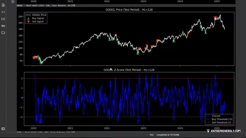
Show Buy and Sell Signals on the Test Set
Now that we have optimized the EWMA Z-score factor and selected the best half-life for each stock, the next step is to apply it to the test dataset.
This will allow us to evaluate how well the factor performs in an out-of-sample environment.
					# --- Evaluate the strategy on the test set --- #
for ticker in tickers:
    final_hl = best_half_life[ticker]
    zscore_test = compute_zscore(test_returns[ticker], final_hl)

    # Identify buy/sell signals
    buy_signals = zscore_test < -THRESHOLD
    sell_signals = zscore_test > THRESHOLD

    # Compute performance
    test_perf = strategy_performance(test[ticker], zscore_test, THRESHOLD)
    print(f"{ticker} - Best Half-Life: {final_hl}, Test Return: {test_perf:.2%}")

    # --- Plot results --- #
    fig, axes = plt.subplots(nrows=2, figsize=(14, 8), sharex=True)

    # Price plot
    axes[0].plot(test[ticker], label=f"{ticker} Price", color='white')
    axes[0].scatter(test.index[buy_signals], test[ticker][buy_signals],
                    label="Buy Signal", marker="^", color='green', alpha=1, s=100)
    axes[0].scatter(test.index[sell_signals], test[ticker][sell_signals],
                    label="Sell Signal", marker="v", color='red', alpha=1, s=100)
    axes[0].set_title(f"{ticker} Price (Test Period) - HL={final_hl}")
    axes[0].legend()

    # Z-score plot
    axes[1].plot(zscore_test, color='blue', label="Z-Score")
    axes[1].axhline(-THRESHOLD, linestyle="--", color="green", alpha=0.7, label=f"Buy Threshold (-{THRESHOLD})")
    axes[1].axhline(THRESHOLD, linestyle="--", color="red", alpha=0.7, label=f"Sell Threshold ({THRESHOLD})")
    axes[1].set_title(f"{ticker} Z-Score (Test Period) - HL={final_hl}")
    axes[1].legend()

    plt.tight_layout()
    plt.show()
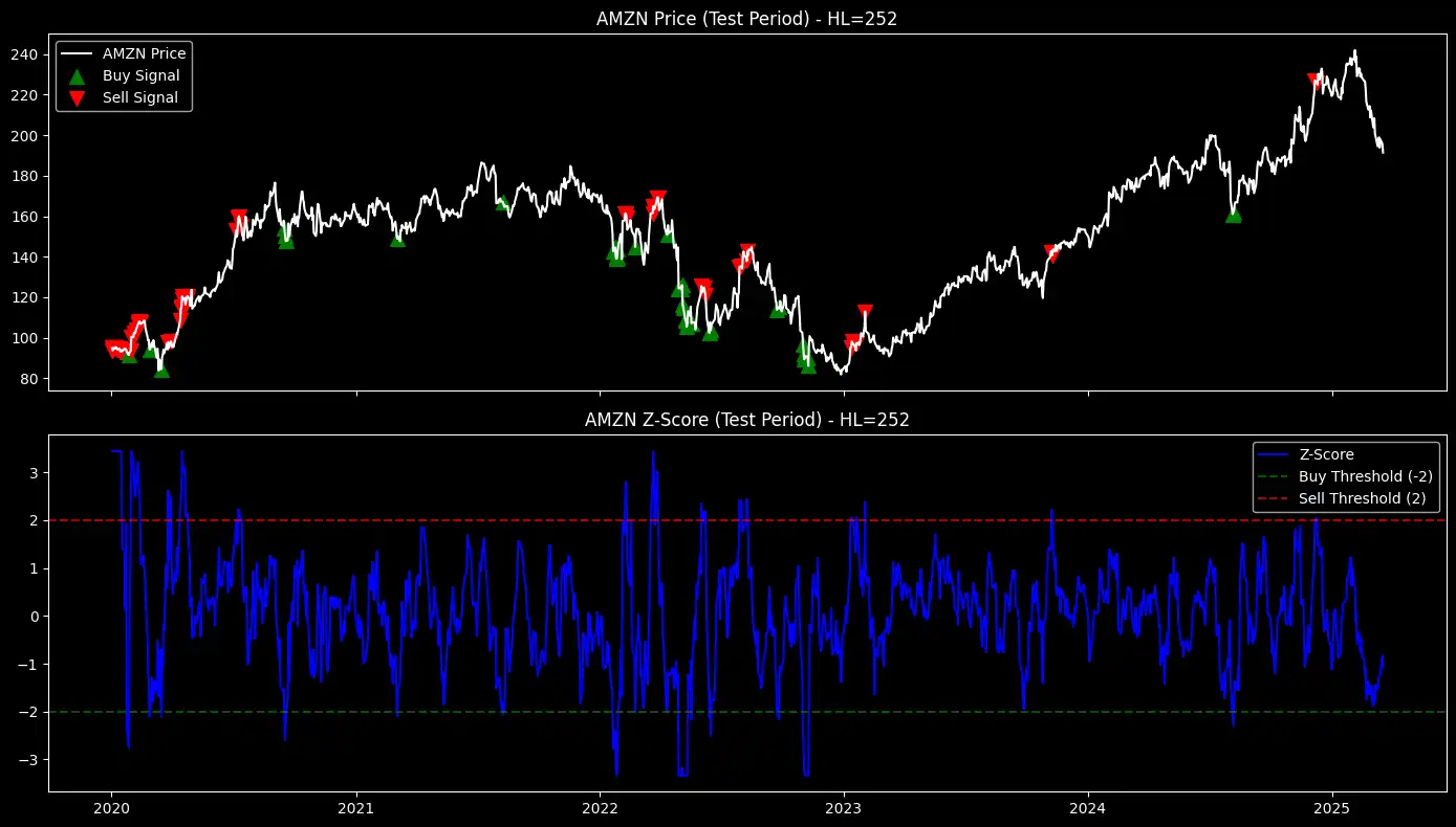
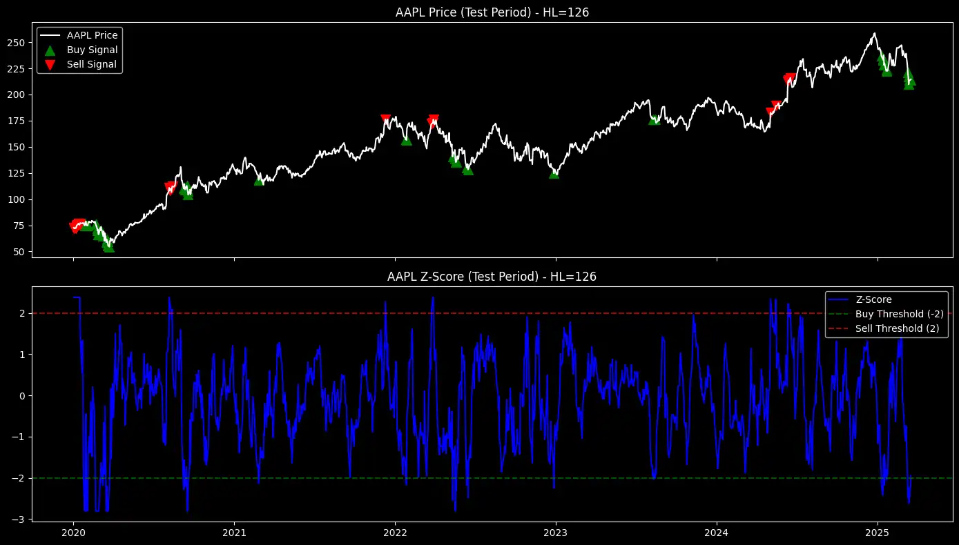
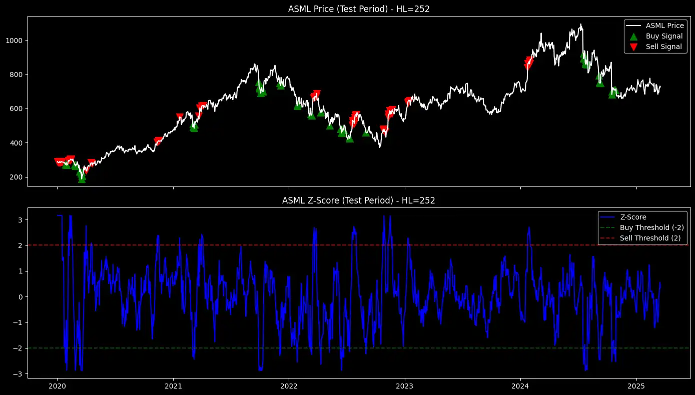
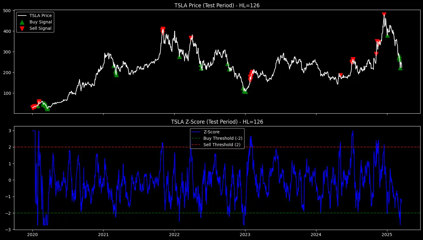
Figure 1: EWMA-based mean-reversion strategy - buy and sell signals overlaid on stock prices (top) and corresponding Z-scores with thresholds (bottom) for multiple stocks during the test period.
3. Creating a Z-Score Dataset for Factor Analysis
Factor analysis requires structured, cross-sectional data to evaluate how signals perform across different stocks.
To achieve this, we transform our Z-score calculations into a dataset suitable for factor research.
This dataset serves two key purposes:
- Standardized Factor Storage → Ensures each stock’s Z-score is stored alongside its price and timestamp.
- Preparation for Alphalens Analysis → Allows for ranking stocks into quantiles and computing forward returns for predictive evaluation.
Z-Score Dataset with Prices
We format the dataset with the following columns:
- Date: Timestamp for each observation.
- Ticker: Stock symbol.
- Price: The stock’s closing price.
- Z-Score: Computed EWMA-based Z-score for mean-reversion analysis.

Newsletter