Setting Volatility-Based Stop Losses with Optimized Paramaters
While knowing when to enter a trade position matters, knowing when to exit if things go wrong is even more important. Without stop-losses, recovering from losses requires more profit to break-even. Enter Dynamic stop-losses.
Setting a stop-loss allows traders to manage risk by defining the maximum loss they are willing to accept. Additionally, using dynamic stop-losses can further enhance risk management by adjusting the stop level as the market moves. This prevents emotional decision-making and reduces stress.
In this article, we implement dynamic volatility-based stop-losses and optimize the input parameters using both Bayesian and walk-forward optimization. Furthermore, the methodology is designed to find the optimal stop-losses across different market scenarios. A Google Notebook is provided for end-to-end implementation.
This article is structured as follows:
- Importance of Stop-Losses
- Theory and Application of
- Bayesian Optimization
- Walk-forward Optimization
- Volatility-Based Dynamic Stop-Losses
- Python Implementation
- Other Stop-Losses Techniques
1. Importance of Stop Losses
A notable case of bad risk management practise is the infamous ‘London Whale’ incident involving JPMorgan Chase in 2012. The firm faced over $6 billion in losses due to a series of bad trades in credit derivatives. Analysts argue that better risk management practices, including the use of stop-losses, could have mitigated these massive losses. The absence of stop-losses allowed the positions to deteriorate significantly before corrective actions were taken (The Guardian, Henricodolfing, Yale).
Another case is that of Lehman Brothers during the 2008 financial crisis, where the firm continued to hold onto toxic assets instead of cutting losses early. This led to its eventual bankruptcy. Implementing stop-losses on their high-risk mortgage-backed securities could have prevented such significant losses by forcing the firm to sell off deteriorating assets before they became worthless (Wikipedia).
During the 2020 oil price crash, many oil companies saw their stock prices plummet. Companies like Whiting Petroleum filed for bankruptcy after failing to manage the massive drop in oil prices effectively. Proper use of stop-losses could have minimized the financial damage by selling off positions before the prices hit rock bottom (Forbes, Bloomberg).
2. Volatility-Based Stop Losses
Recent academic research on volatility-based stop-loss strategies has highlighted their effectiveness in managing risk and enhancing portfolio performance. Studies indicate that traditional stop-loss rules may not always work optimally, particularly in markets characterized by random walk price movements.
However, volatility stop-losses, which adjust based on the asset’s volatility, have shown promise in improving returns, especially in trending markets where price momentum is present. Research suggests that these strategies can help mitigate losses while maintaining a balance between risk and return, although their success heavily relies on the correct calibration of input parameters, such as the safety multiple used in their calculation (SpringerLink)(ar5iv).
Average True Range (ATR)
A common approach to set volatility-based stop-losses is to rely on the Average True Range, which measures market volatility. The ATR is calculated using the following formula:
Where:
- n is the number of periods (commonly 14).
- TRi is the True Range for each period.
The True Range (TR) is the greatest of the following:
- Current high minus current low.
- Absolute value of the current high minus the previous close.
- Absolute value of the current low minus the previous close.
A stop-loss might be set at as a multiple of the ATR value:
Traders first calculate the Average True Range (ATR) for their asset and decide on a suitable multiplier based on their risk tolerance. For instance, if the ATR is $1.50 and the trader chooses a multiplier of 2, the stop-loss would be set at $3 below the closing price for a long position or $3 above for a short position.
During the COVID-19 pandemic, extreme market volatility affected stocks like Zoom, which saw rapid price increases. Consequently, traders using volatility-based stop-losses might have set wider stop-losses for Zoom during high volatility to avoid being stopped out by normal market fluctuations.
3. Bayesian Optimization
Bayesian optimization can be used for optimizing complex functions that are expensive to evaluate. It is particularly useful in trading for finding the optimal parameters for strategies which require computationally intensive operations.
For example, Algorithmic traders use Bayesian optimization to fine-tune their algorithms. It helps in selecting the best parameters for algorithms that trade based on moving averages, mean reversion, or momentum strategies, etc.
Bayesian optimization uses a probabilistic model to approximate the objective function. This model guides the search for the optimal parameters by balancing exploration (trying new parameters) and exploitation (refining known good parameters).
Process
1. Define the Objective Function: The first step is to define the objective function f(x), which is the function we want to optimize. In trading, this could be the return of a strategy based on certain parameters.
2. Choose a Surrogate Model: Typically, a Gaussian process (GP) is used as the surrogate model. The GP provides a probability distribution over possible functions that fit the observed data.
μ(x) is the mean function and k(x,x′) is the covariance function.
3. Acquisition Function: The acquisition function determines the next point to evaluate by balancing exploration and exploitation. Common acquisition functions include Expected Improvement (EI) and Upper Confidence Bound (UCB).
x+ is the current best observation.
4. Iterate: Evaluate the objective function at the chosen point, update the surrogate model with the new data, and repeat until convergence.
In other words, Bayesian optimization efficiently identifies optimal parameters by combining exploration of new options and improvement of existing ones.
Benefits
Efficiency: Bayesian optimization is efficient in finding the global optimum with fewer evaluations compared to traditional grid search or random search methods.
Adaptability: It adapts to complex, noisy, and expensive-to-evaluate functions. This makes it ideal for trading strategies that require extensive backtesting.
Flexibility: The method is flexible and can incorporate prior knowledge about the problem to improve the optimization process.
4. Walk-Forward Optimization
Walk-forward optimization helps in validating and improving trading strategies over time. It ensure that a strategy performs well in various market conditions, avoiding overfitting to historical data. This technique is especially useful for implementing dynamic stop-losses, as it continuously adapts to new data.
Walk-forward optimization involves repeatedly optimizing a trading strategy over a rolling window of historical data and then testing the optimized parameters on a subsequent out-of-sample period. This mimics real-world trading, where traders use past data to make future predictions.
Process
1. Divide Data into Segments: Split the historical data into training and testing segments. Typically, the data is divided into overlapping windows, to ensure each segment has both training and testing periods.
2. Optimize on Training Set: Optimize the strategy parameters on the training set to maximize the objective function, such as cumulative returns or Sharpe ratio.
3. Test on Testing Set: Apply the optimized parameters to the testing set to evaluate performance. Record the results and move the window forward.
4. Iterate: Repeat the process for the entire dataset, moving the training and testing windows forward by a fixed step each time
Benefits
Reduces Overfitting: By validating the strategy on out-of-sample data, walk-forward optimization helps prevent overfitting to historical data. This makes it more robust when ensuring the strategy generalizes well to future market conditions.
Adapts to Market Changes: The method continuously adjusts strategy parameters based on recent data. This makes it more responsive to market changes.
Improves Robustness: Strategies optimized with walk-forward analysis tend to be more robust, as they are tested and refined across various market conditions.
5. Dynamic Stop-Losses Methodology
Our approach dynamically sets stop-losses using a combination of technical indicators and a walk-forward optimization technique. Initially, we calculate key indicators such as the Average True Range (ATR), Exponential Moving Averages (EMA), Moving Average Convergence Divergence (MACD), and Relative Strength Index (RSI) to signal entries.
Next, we set the stop-loss as a multiple of the ATR. This threshold is dynamic and undergoes optimization through Bayesian Optimization. We identify the best ATR multiplier and window size by maximizing cumulative returns in a backtest.
Furthermore, walk-forward optimization refines this process by repeatedly training and testing the model on different data segments. This ensures accurate parameter selection, accounting for changing market conditions and aiming to maintain consistent performance. Finally, we adjust the strategy signals for a minimum holding period.
6. Python Implementation
Let’s now dive into the most interesting section, the implementation. We’ll go step-by-step. First, we present a very simple implemention of using ATR-based Stop-losses.
Next, we aim to derive the best parameters for an ATR-based Stop-losses strategy. We derive the best stop-losses thresholds by maximising the cumulative returns if the thresholds were to be hit.
We further compare our strategy against one that does not use stop-losses, relying instead on entry and exit signals generated by technical indicators.
6.1 Simple ATR-Based Stop Losses
The script below fetches data, computeS the ATR, and setS dynamic stop-losses. The stop losses adjust based on market volatility. While this implementation provides a dynamic approach, it is not optimized for the best parameters. Optimization will be addressed next.
					import warnings
import yfinance as yf
import numpy as np
import pandas as pd
import matplotlib.pyplot as plt

warnings.filterwarnings('ignore')

def fetch_data(symbol, start, end):
    data = yf.download(symbol, start=start, end=end)
    if data.empty:
        raise ValueError("No data fetched.")
    return data

def calculate_atr(data, atr_window):
    data['TR'] = np.maximum((data['High'] - data['Low']),
                            np.maximum(abs(data['High'] - data['Close'].shift(1)),
                                       abs(data['Low'] - data['Close'].shift(1))))
    data['ATR'] = data['TR'].rolling(window=atr_window).mean()
    return data

def calculate_stop_loss(data, atr_multiplier):
    data['Buy_Stop_Loss'] = data['Close'] - (data['ATR'] * atr_multiplier)
    data['Sell_Stop_Loss'] = data['Close'] + (data['ATR'] * atr_multiplier)
    return data

def plot_atr_boundaries(data, symbol, atr_multiplier):
    plt.figure(figsize=(14, 7))
    plt.plot(data['Close'], label='Close Price', color='blue')
    plt.plot(data['Buy_Stop_Loss'], label=f'Buy Stop Loss (ATR x {atr_multiplier})', linestyle='--', color='red')
    plt.plot(data['Sell_Stop_Loss'], label=f'Sell Stop Loss (ATR x {atr_multiplier})', linestyle='--', color='green')

    # Adding annotations for the last values
    last_close = data['Close'].iloc[-1]
    last_buy_sl = data['Buy_Stop_Loss'].iloc[-1]
    last_sell_sl = data['Sell_Stop_Loss'].iloc[-1]

    plt.text(data.index[-1], last_close, f'Last Close: {last_close:.2f}', color='blue', ha='right')
    plt.text(data.index[-1], last_buy_sl, f'Buy SL: {last_buy_sl:.2f}', color='red', ha='right')
    plt.text(data.index[-1], last_sell_sl, f'Sell SL: {last_sell_sl:.2f}', color='green', ha='right')

    plt.title(f'{symbol} ATR Boundaries')
    plt.xlabel('Date')
    plt.ylabel('Price')
    plt.legend()
    plt.show()

# Main execution
symbol = 'ASML'
start_date = '2022-01-01'
end_date = '2025-01-01'
atr_multiplier = 3
atr_window = 50

data = fetch_data(symbol, start_date, end_date)

if not data.empty:
    data = calculate_atr(data, atr_window)
    data = calculate_stop_loss(data, atr_multiplier)
    plot_atr_boundaries(data, symbol, atr_multiplier)
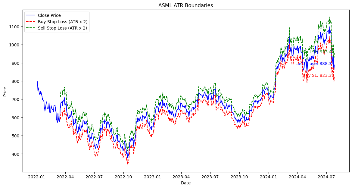
Figure. 1: ASML price plot with dynamic stop-losses set at twice the ATR. The blue line is the close price, while the red and green dashed lines represent the buy and sell stop-losses, respectively.
Also worth reading:
Top 36 Moving Average Methods For Stock Prices in Python

Newsletter