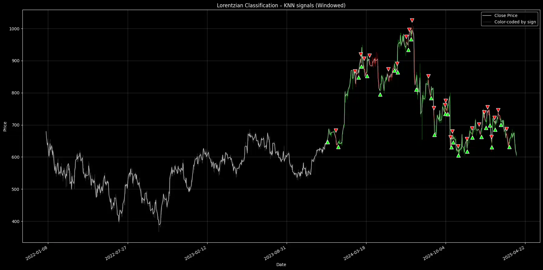
Matching Historical Price Patterns with a 5-Feature Input and Lorentzian Kernel to Classify Trend Direction
Markets rarely repeat, but they sometime echo familiar setups. This article shows how to turn those echoes into trading signals.
In our analysis, we predict short-term price direction by comparing today’s market state to similar conditions in the past.
We use a custom K-nearest neighbors method with Lorentzian distance to track how technical patterns played out historically .
Instead of training a predictive model, we use market memory. We define each bar by a set of technical indicators — RSI, ADX, Wave Trend, and others — then compare recent patterns to hundreds of past ones.
All the variables are adjustable. The result is a fully transparent signal-generation method. No training. No black-box models.

This Article is structured as follows:
- Trading on Pattern Memory Model
- Getting the Data for Pattern Recall
- Feature Engineering with Indicator Functions
- Lorentzian Distance: A Smarter Similarity Measure
- Training Labels and KNN Prediction
End-to-end implementation notebook provided below. Click and Run.
2. Trading on Pattern Memory
Instead of forecasting, we look backward and search for days in the past that resemble the market conditions we’re seeing now. Then we track what happened next in those historical cases.
If similar setups consistently led to price increases, that suggests a possible up move today. If they preceded drops, that signals potential downside.
This idea is known as non-parametric classification — no training, no optimization, no fitted model. Just memory-based reasoning.
2.1 Market States as Feature Vectors
To compare market behavior over time, we need a way to encode each trading day numerically. We do this by calculating five technical indicators from price data:
- Relative Strength Index
- Wave Trend
- Commodity Channel Index
- ADX (trend strength)
- A second RSI with a shorter lookback
Each day becomes a vector in multi-dimensional space:

But instead of looking at just one day, we go further. We use a sliding window of 5 (adjustable) consecutive bars to capture short-term behavior. That gives each observation more context.
So the full feature vector becomes:

Each one is a flattened array of 25 numbers — five indicators over 5 bars. This becomes our representation of a “market state”.
2.2 Measuring Similarity with Lorentzian Distance
To compare today’s pattern with previous ones, we need a distance function.
Instead of using Euclidean distance, which can be thrown off by large deviations , we use Lorentzian distance, defined as:

This function grows slowly as differences increase to be more tolerant of outliers and noise.
In simple terms, Lorentzian measures how similar the shape and magnitude of two market states are, without overreacting to a single volatile spike.
2.3 Find Similar Setups, Watch What Followed
Once we’ve encoded every market state and defined how to measure similarity, the process is simple:
- For today’s vector, compare it to all previous ones within a lookback window (say, the last 200 bars).
- Sort by Lorentzian distance to find the k-nearest past setups (e.g., the closest 100).
- Assign labels based on what happened after those historical bars:
- +1 if price rose within the next 4 bars
- –1 if it fell
- 0 if it was flat
Then, just sum the labels:

If the sum is positive, most similar past setups led to gains. If it’s negative, they led to losses.
This output becomes a directional signal — not based on probability, but on pattern memory.
3. Python Implementation
3.1. Get Data for Pattern Recall
We download daily price data for a given ticker. The data is cleaned and reset so that each row represents one trading bar.
					import numpy as np
import pandas as pd
import yfinance as yf
import matplotlib.pyplot as plt
import matplotlib.dates as mdates

# DOWNLOAD DATA
TICKER     = "ASML.AS"
START_DATE = "2022-01-01"
END_DATE   = "2025-07-01"

df = yf.download(TICKER, start=START_DATE, end=END_DATE, interval="1d")
if df.empty:
    raise ValueError("No data returned from yfinance.")

# Flatten columns if multi-index
if isinstance(df.columns, pd.MultiIndex):
    df.columns = df.columns.get_level_values(0)

# Standard renaming/cleanup
df.rename(columns={"Open":"Open","High":"High","Low":"Low","Close":"Close","Volume":"Volume"}, inplace=True)
df.dropna(subset=["Close","High","Low"], inplace=True)
df["Date"] = df.index
df.reset_index(drop=True, inplace=True)
n = len(df)
3.2. Feature Engineering with Indicator Functions
We compute five technical indicators from the price series. These serve as the features for comparing one market state to another.
Each indicator captures a different dimension of market structure — momentum, volatility, trend strength, and deviation.
Here’s how they’re defined:
3.2.1 Relative Strength Index
RSI measures momentum by comparing the magnitude of recent gains to recent losses. It’s defined as:

where RS is the ratio of average gains to average losses over the last 14 bars.
3.2.2. Wave Trend Oscillator
Wave Trend is a smoothed oscillator based on the average price of each bar. It filters out noise using exponential moving averages:

Here

and ESA is the EMA of hlc3.
3.2.3. Commodity Channel Index
CCI measures how far price deviates from its moving average:

MA is the 20-bar moving average, and MD is the mean deviation from that average.
3.2.4. Average Directional Index
ADX quantifies trend strength. It’s based on directional movement indicators:

These are combined into the directional index:

ADX is the EMA of DX over 14 bars. The higher it is, the stronger the trend.
3.2.5. Short-Term RSI
We also include a second RSI, calculated over just 9 bars, to capture faster momentum shifts.

Newsletter