Back To Top

June 8, 2024

Bootstrapping Future Price Movements Probabilities

How Bootstrap and Historical Simulations Help Predict Future Market Prices

Estimating future price movements with bootstrapping is a powerful technique for financial forecasting. By leveraging historical data and simulation methods, investors can estimate potential future stock price changes and their associated probabilities.

This article explores how bootstrapping and historical simulations help estimate potential future market prices. Furthermore, we provide a comprehensive understanding of their applications and an end-to-end implementation, available on Google Colab.

2. Bootstrapping Simulation

Bootstrapping is a statistical technique that involves resampling with replacement from an original dataset to create many simulated samples. Replacement means that each time you pick a data point from your dataset, you put it back before the next pick. 

This method allows us to estimate the distribution of a statistic (e.g., mean, variance) by sampling from the data repeatedly. It is particularly useful when the theoretical distribution of the statistic is complex or unknown.

Background and Concept

The concept of bootstrapping was introduced by Bradley Efron in 1979. The primary goal of bootstrapping is to understand the variability of a statistic by generating multiple samples from the observed data.

This approach assumes that the sample data represents the population, allowing us to draw inferences about the population from the sample. 

Steps in Bootstrapping:

1. Original Sample: Start with the original dataset of size , denoted as:

The original dataset containing 𝑛 observations.

2. Resampling: Randomly draw samples of size from with replacement. This means that each data point can be selected multiple times in a single resample.

3. Statistic Calculation: For each resample, calculate the statistic of interest (e.g., mean, median, standard deviation).

4. Repetition: Repeat the resampling and calculation process times to create a distribution of the statistic.

5. Estimation: Use the distribution of the statistic from the resamples to estimate its properties, such as mean, standard error, and confidence intervals.

Mathematical Formulation

Given a dataset

The original dataset containing 𝑛 observations.

we aim to estimate the statistic θ (e.g., the mean return of a stock).

1. Resampling: Create a resample X* by drawing observations from X with replacement:

A resampled dataset (with replacement) of size 𝑛 from the original dataset X

2. Statistic Calculation: Calculate the statistic θ* for the resample

The calculated statistic based on the resampled dataset

3. Repeat: Repeat the above steps times to generate bootstrap statistics

A collection of B bootstrap estimates of the statistic 𝜃, each derived from a different resampled dataset 𝑋∗

4. Estimate: Use the bootstrap statistics to estimate the mean, standard error, and confidence intervals of

Future Stock Price Esimation

In the context of stock price prediction, the bootstrapping simulation involves resampling daily returns to simulate future price paths. Here’s how it works in detail:

1. Daily Returns Calculation: Calculate the daily returns of the stock:

Daily return calculation

where is the price at time .

2. Resampling Returns: Randomly sample daily returns with replacement to generate a simulated sequence of returns for days.

3. Price Path Simulation: Compute the cumulative product of the sampled returns to simulate the stock price path:

Simulated future stock price calculation

where is the simulated price on day for simulation , and is the initial stock price.

4. Multiple Simulations: Repeat the resampling and price path simulation process times to create a distribution of simulated final prices.

Bootstrapping Future Price Movements Probabilities Demo GIF Entreprenerdly

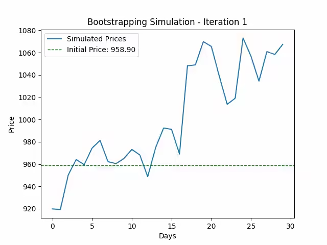
Figure. 1: Bootstrap Simulation: This GIF illustrates the bootstrap simulation process for predicting future stock prices. Each frame shows a new simulated price path generated by resampling historical daily returns with replacement.

Implications in Finance

In finance, bootstrapping is particularly useful for modeling stock prices, as it allows analysts to:

  1. Estimate Confidence Intervals: By generating multiple simulated price paths, bootstrapping helps estimate the confidence intervals for future stock prices.

  2. Assess Risk and Return: Bootstrapping can help assess the risk and return profile of an investment by analyzing the distribution of simulated returns. 

  3. Scenario Analysis: It enables scenario analysis by simulating various future outcomes based on historical data. Investors can evaluate the impact of different market conditions on their portfolio.

  4. Portfolio Optimization: Bootstrapping helps in portfolio optimization by providing insights into the expected performance and risk of different assets. 

3. Historical Simulation

Historical simulation is a method used to estimate the future behavior of stock prices based on historical returns. Unlike bootstrapping, which resamples the returns with replacement, historical simulation involves shuffling the actual historical returns without replacement to create potential future price paths.

Background and Concept

The historical simulation method assumes that the past behavior of a stock’s price can provide insights into its future movements. By using actual historical returns, this method preserves the inherent characteristics and distribution of the observed data. This approach is particularly useful for capturing the historical patterns and volatility of the stock.

Steps in Historical Simulation:

1. Original Sample: Start with the historical returns of the stock, denoted as

The original set of daily returns calculated from the historical stock prices.

where represents the return at time .

2. Shuffling: Randomly shuffle the historical returns to generate a new sequence of returns.

3. Price Path Simulation: Calculate the cumulative product of the shuffled returns to simulate the stock price path for the desired period.

4. Repetition: Repeat the shuffling and price path simulation process multiple times to create a distribution of simulated final prices.

Mathematical Formulation

Given a dataset of historical returns

The original set of daily returns calculated from the historical stock prices.

the goal is to estimate future prices by creating new sequences of returns through shuffling.

1. Shuffling Returns: Randomly permute the historical returns to generate a shuffled sequence

A resampled set of daily returns created by randomly selecting from the original returns with replacement.

2. Price Path Simulation: Compute the cumulative product of the shuffled returns to simulate the stock price path:

Simulated future stock price calculation

where is the simulated price on day tt for simulation ii, and is the initial stock price

3. Multiple Simulations: Repeat the shuffling and price path simulation process times to generate a distribution of simulated final prices.

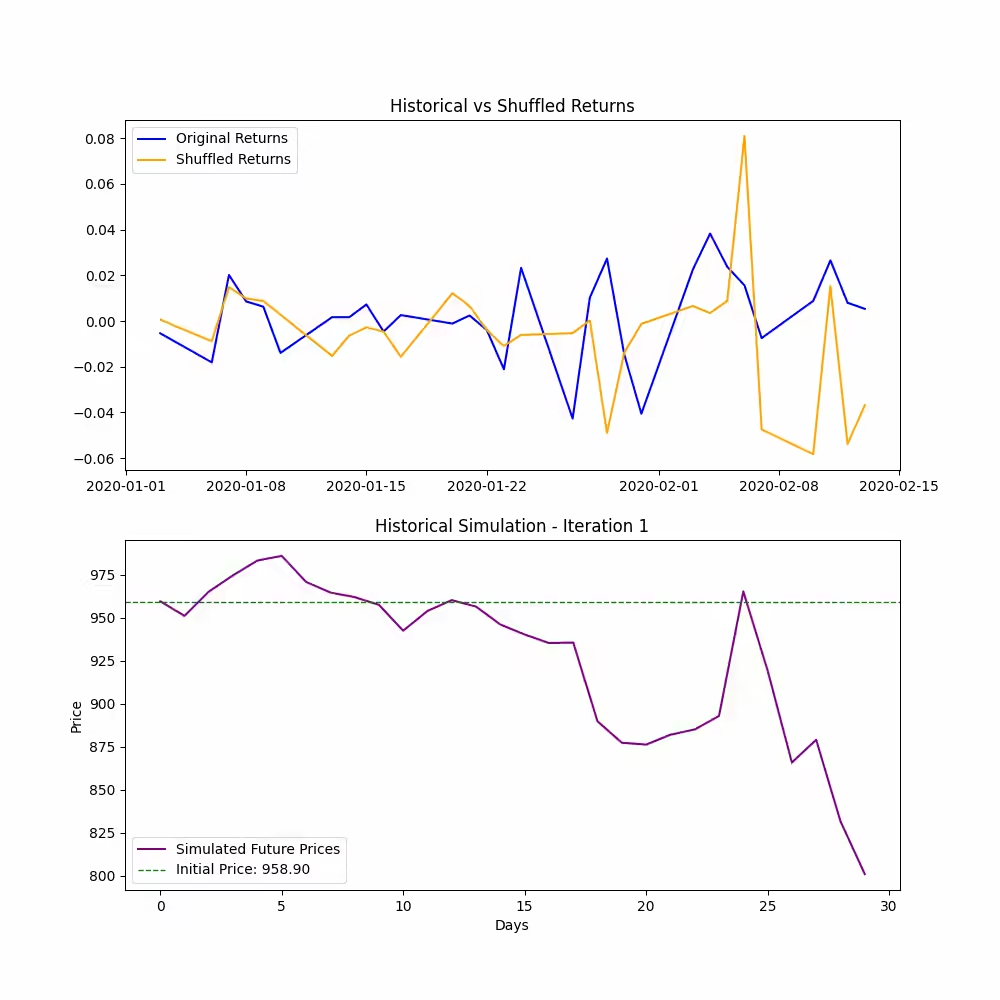
Figure. 2: Historical Simulation: This GIF demonstrates the historical simulation approach for forecasting stock prices. Each frame compares original historical returns to shuffled returns and shows the resulting simulated price path. The process preserves the actual distribution of returns while generating potential future scenarios.

4. Python Implementation

Fetching Stock Data

To start our analysis, we need historical stock price data. The yfinance library helps us fetch this data easily. Here is a function to get the closing prices of a given stock within a specified date range:

				
					import yfinance as yf
import numpy as np
import matplotlib.pyplot as plt

# Function to fetch stock data from Yahoo Finance
def get_stock_data(ticker, start_date, end_date):
    # Download stock data within the specified date range
    stock_data = yf.download(ticker, start=start_date, end=end_date)
    # Return the closing prices of the stock
    return stock_data['Close']


Bootstrapping Simulation

As mentioned before, bootstrapping involves resampling with replacement from historical daily returns to create multiple simulated future price paths. Here’s how we can implement this:

				
					# Bootstrapping simulation function
def bootstrap_simulation(data, days, n_iterations=10000):
    # Calculate daily returns and remove any missing values
    daily_returns = data.pct_change().dropna()
    # Initialize a matrix to store the simulation results
    simulations = np.zeros((n_iterations, days))

    # Perform the bootstrapping simulation
    for i in range(n_iterations):
        # Randomly sample daily returns with replacement
        sample = np.random.choice(daily_returns, size=days, replace=True)
        # Calculate the cumulative product of the sampled returns and scale by the last known price
        simulations[i] = np.cumprod(1 + sample) * data.iloc[-1]

    # Return the simulation results
    return simulations


Historical Simulation

Historical simulation shuffles actual historical returns without replacement to generate future price paths. Here’s the implementation:

				
					# Historical simulation function
def historical_simulation(data, days, n_iterations=10000):
    # Calculate daily returns and remove any missing values
    daily_returns = data.pct_change().dropna()
    # Initialize a matrix to store the simulation results
    simulations = np.zeros((n_iterations, days))

    # Perform the historical simulation
    for i in range(n_iterations):
        # Shuffle the historical daily returns
        shuffled_returns = np.random.permutation(daily_returns)
        # Select the first 'days' returns from the shuffled returns
        sample = shuffled_returns[:days]
        # Calculate the cumulative product of the shuffled returns and scale by the last known price
        simulations[i] = np.cumprod(1 + sample) * data.iloc[-1]

    # Return the simulation results
    return simulations


Also worth reading:

Assessing Future Stock Price Movements With Historical & Implied Volatility

Prev Post

Can YOLO Predict Stock Market Ups and Downs?

Next Post

Fine-tuning Idefics2 VLM for Document VQA

post-bars
Mail Icon

Newsletter

Get Every Weekly Update & Insights

[mc4wp_form id=]

Leave a Comment