A Close Look at the Current Economic Landscape and Health
Economic recession indicators are flashing warning signs. Top analysts, investors, and policymakers are debating whether we are currently in or heading into a recession. Recent economic indicators in the United States suggest a recession early next year is unavoidable. Let’s explore this possibility quantitatively and qualitatively.
In this article, we’ll take a proactive approach to evaluating the current economic landscape in relation to the likelihood of a recession. We’ll analyze key economic recession indicators, historical stock market patterns, and employ topological data analysis to estimate the likelihood of market crashes. We’ll also examine what major financial and economic analysts are saying about the current state of the US economy.
This article is structured as follows:
- Time Series Analysis of Key Economic Indicators during Recessions
- Historical of Market Drops During Recessions (and ‘No Recessions’)
- Yield Curve Analysis and Current Short vs Long-Term Spreads
- Analysis Reports and News From Major Outlets
- Using Topology To Estimate Market Crash Events
1. Key Economic Indicators
Let’s get started by collecting key economic indicators for the U.S economy. We’ll primarly use the Federal Reserve Economic Data (FRED) database. The key indicators include the Sahm Recession Indicator, retail sales, industrial production, unemployment rate, inflation, nonfarm payrolls, jobless claims, consumer confidence, housing starts, and various Treasury yields. These indicators collectively provide a good picture of of the health of the economy (Conference Board, St. Louis Fed).
1.1 Sahm Recession Indicator
The Sahm Recession Indicator, created by Claudia Sahm, predicts recessions using economic data. It suggests recessions often start with a drop in economic growth, a rise in unemployment, and reduced consumer spending.
The Sahm Recession Indicator signals the start of a recession when the three-month moving average of the national unemployment rate (U3) rises by 0.50 percentage points or more relative to its low during the previous 12 months (Hamilton Project).
The indicator is formulated formally as:

1.2 Recession Probabilities
The National Bureau of Economic Research (NBER) often provides recession probabilities. These are estimated using a dynamic-factor Markov-switching model. This approach incorporates several key economic indicators, including industrial production, non-farm payroll employment, real personal income, and trade sales, to estimate the likelihood of a recession. (Marcelle Chauvet, 1998)
The probability model can be described as including both dynamic factors and a regime switching components.
Dynamic Factor Model
The dynamic factor model assumes that a vector of macroeconomic variables ΔYit can be decomposed into a common factor ΔFt and idiosyncratic components Δvit. The dynamic factor ΔFt represents the common cyclical movements of the macroeconomic variables.
Here:
- ΔYit is the vector of macroeconomic variables.
- λi(L) is a lag polynomial that captures the response of ΔYit to the common factor ΔFt.
- ΔFt is the common dynamic factor.
- Δvit is the idiosyncratic component.
Regime Switching
The regime switching aspect of the model captures the transitions between different phases of the business cycle, such as expansions and contractions. This is modeled using a Markov process with states St=0,1, where each state represents different phases of the business cycle. The dynamic factor ΔFt is subject to discrete regime shifts, which can be described as:
Where:
- α2 are constants that capture the effect of the regime state on the dynamic factor.
- ϕ(L) is a lag polynomial.
- ηst is an error term that follows a state-dependent distribution.
The states St follow a Markov process with transition probabilities:
Where pij are the probabilities of transitioning from state i to state j.
Estimation
The model estimation involves the following steps:
Nonlinear Filtering: The state vector is tracked using observations on ΔYt. This involves computing one-step-ahead predictions and updates of the state vector and error matrices. The Kalman Gain is used to update the state vector and error matrices based on new information.
Likelihood Maximization: The likelihood function is evaluated at each time t using the outputs from the nonlinear filter. The log-likelihood function is then maximized with respect to the model parameters using a nonlinear optimization algorithm.
State Probability Calculation: The probabilities associated with the latent Markov state are calculated, allowing for the estimation of the likelihood of being in a recession state
Final Model Representation
Without going into much more detail, the final model can be more easily interpreted as follows.
The final probability of being in a recession state Y=1 at time t is given by:
Here, iΦ is the cumulative distribution function of the standard normal distribution. β0,β1,…,βk are the estimated coefficients. X1,X2,…,Xk are the observed economic indicators.
The code below gathers all the indicator data. It plots this data over time and highlights recession periods using dates from NBER’s recorded recession periods.
import pandas_datareader.data as web
import yfinance as yf
import datetime
import matplotlib.pyplot as plt
import matplotlib.dates as mdates

# Define the start and end date
start_date = datetime.datetime(1920, 1, 1)
end_date = datetime.datetime.today()
extended_end_date = end_date + datetime.timedelta(days=120)

# Fetch the data from FRED
sahm_recession_indicator = web.DataReader('SAHMREALTIME', 'fred', start_date, end_date)
retail_sales = web.DataReader('RSXFS', 'fred', start_date, end_date)
industrial_production = web.DataReader('INDPRO', 'fred', start_date, end_date)
unemployment_rate = web.DataReader('UNRATE', 'fred', start_date, end_date)
inflation = web.DataReader('CPIAUCSL', 'fred', start_date, end_date)
nonfarm_payrolls = web.DataReader('PAYEMS', 'fred', start_date, end_date)
jobless_claims = web.DataReader('ICSA', 'fred', start_date, end_date)
consumer_confidence = web.DataReader('UMCSENT', 'fred', start_date, end_date)
housing_starts = web.DataReader('HOUST', 'fred', start_date, end_date)
treasury_rate_10y = web.DataReader('GS10', 'fred', start_date, end_date)
treasury_rate_2y = web.DataReader('DGS2', 'fred', start_date, end_date)  # 2-year Treasury yield
treasury_rate_1m = web.DataReader('DGS1MO', 'fred', start_date, end_date)  # 1-month Treasury yield
treasury_rate_3m = web.DataReader('TB3MS', 'fred', start_date, end_date)  # 3-month Treasury yield
federal_funds_rate = web.DataReader('FEDFUNDS', 'fred', start_date, end_date)
recession_probabilities = web.DataReader('RECPROUSM156N', 'fred', start_date, end_date)

# Rename columns for clarity
recession_probabilities.columns = ['Recession_Probabilities']

# Fetch the data from Yahoo Finance
sp500 = yf.download('^GSPC', start=start_date, end=end_date)['Adj Close']
vix = yf.download('^VIX', start=start_date, end=end_date)['Adj Close']

# Calculate percentage changes for relevant indicators
industrial_production_pct = industrial_production.pct_change() * 100
inflation_pct = inflation.pct_change() * 100

# Rename columns for clarity
industrial_production_pct = industrial_production_pct.rename(columns={'INDPRO': 'INDPRO_PCT'})
inflation_pct = inflation_pct.rename(columns={'CPIAUCSL': 'CPIAUCSL_PCT'})

# Combine all data into a single DataFrame, aligning by date
combined_data = sahm_recession_indicator.join([
    retail_sales, industrial_production, industrial_production_pct,
    unemployment_rate, inflation, inflation_pct,
    sp500.rename('SP500'), nonfarm_payrolls, jobless_claims,
    consumer_confidence, housing_starts, treasury_rate_10y, treasury_rate_2y, treasury_rate_1m, treasury_rate_3m, federal_funds_rate, vix.rename('VIX'),
    recession_probabilities
], how='outer')

# Interpolate missing values for alignment
combined_data = combined_data.interpolate(method='time')

# Calculate the yield spread
combined_data['Yield_Spread'] = combined_data['GS10'] - combined_data['DGS2']

# Define major stock market crash periods
crash_periods = {
    '1857-06-01': '1858-12-01',
    '1860-10-01': '1861-06-01',
    '1865-04-01': '1867-12-01',
    '1869-06-01': '1870-12-01',
    '1873-10-01': '1879-03-01',
    '1882-03-01': '1885-05-01',
    '1887-03-01': '1888-04-01',
    '1890-07-01': '1891-05-01',
    '1893-01-01': '1894-06-01',
    '1895-12-01': '1897-06-01',
    '1899-06-01': '1900-12-01',
    '1902-09-01': '1904-08-01',
    '1907-05-01': '1908-06-01',
    '1910-01-01': '1912-01-01',
    '1913-01-01': '1914-12-01',
    '1918-08-01': '1919-03-01',
    '1920-01-01': '1921-07-01',
    '1923-05-01': '1924-07-01',
    '1926-10-01': '1927-11-01',
    '1929-08-01': '1933-03-01',
    '1937-05-01': '1938-06-01',
    '1945-02-01': '1945-10-01',
    '1948-11-01': '1949-10-01',
    '1953-07-01': '1954-05-01',
    '1957-08-01': '1958-04-01',
    '1960-04-01': '1961-02-01',
    '1969-12-01': '1970-11-01',
    '1973-11-01': '1975-03-01',
    '1980-01-01': '1980-07-01',
    '1981-07-01': '1982-11-01',
    '1990-07-01': '1991-03-01',
    '2001-03-01': '2001-11-01',
    '2007-12-01': '2009-06-01',
    '2020-02-01': '2020-04-01'
}

# Create subplots
fig, axes = plt.subplots(nrows=15, ncols=1, figsize=(15, 70), sharex=True)

# Plot each series
plot_data = [
    ('SAHMREALTIME', 'Sahm Recession Indicator'),
    ('Recession_Probabilities', 'Smoothed U.S. Recession Probabilities'),
    ('Yield_Spread', 'Yield Spread (10Y - 2Y)'),
    ('SP500', 'Stock Market (S&P 500)'),
    ('VIX', 'VIX'),
    (('GS10', 'DGS2', 'DGS1MO', 'TB3MS'), 'Treasury Rates'),
    ('FEDFUNDS', 'Federal Funds Rate'),
    ('UNRATE', 'Unemployment Rate'),
    ('PAYEMS', 'Nonfarm Payrolls'),
    ('ICSA', 'Jobless Claims'),
    ('RSXFS', 'Retail Sales'),
    (('INDPRO', 'INDPRO_PCT'), 'Industrial Production'),
    ('HOUST', 'Housing Starts'),
    ('UMCSENT', 'Consumer Confidence'),
    (('CPIAUCSL', 'CPIAUCSL_PCT'), 'Inflation (CPI)')
]

for i, (column, title) in enumerate(plot_data):
    if isinstance(column, tuple):
        if column == ('INDPRO', 'INDPRO_PCT'):
            # Plot industrial production and its percentage change on dual y-axes
            ax1 = axes[i]
            ax2 = ax1.twinx()

            abs_col, pct_col = column
            color1, color2 = 'blue', 'red'

            ax1.plot(combined_data.index, combined_data[abs_col], color=color1, label=abs_col)
            ax2.plot(combined_data.index, combined_data[pct_col], color=color2, label=f'{pct_col} (%)')

            ax1.set_ylabel(abs_col, color=color1)
            ax2.set_ylabel(f'{pct_col} (%)', color=color2)

            ax1.tick_params(axis='y', labelcolor=color1)
            ax2.tick_params(axis='y', labelcolor=color2)

            lines1, labels1 = ax1.get_legend_handles_labels()
            lines2, labels2 = ax2.get_legend_handles_labels()
            ax1.legend(lines1 + lines2, labels1 + labels2, loc='upper left')
        elif column == ('CPIAUCSL', 'CPIAUCSL_PCT'):
            # Plot inflation and its percentage change on dual y-axes
            ax1 = axes[i]
            ax2 = ax1.twinx()

            abs_col, pct_col = column
            color1, color2 = 'blue', 'red'

            ax1.plot(combined_data.index, combined_data[abs_col], color=color1, label=abs_col)
            ax2.plot(combined_data.index, combined_data[pct_col], color=color2, label=f'{pct_col} (%)')

            ax1.set_ylabel(abs_col, color=color1)
            ax2.set_ylabel(f'{pct_col} (%)', color=color2)

            ax1.tick_params(axis='y', labelcolor=color1)
            ax2.tick_params(axis='y', labelcolor=color2)

            lines1, labels1 = ax1.get_legend_handles_labels()
            lines2, labels2 = ax2.get_legend_handles_labels()
            ax1.legend(lines1 + lines2, labels1 + labels2, loc='upper left')
        elif column == ('GS10', 'DGS2', 'DGS1MO', 'TB3MS'):
            # Plot multiple Treasury rates in the same subplot
            ax = axes[i]
            colors = ['blue', 'red', 'green', 'purple']
            for j, col in enumerate(column):
                combined_data[col].plot(ax=ax, color=colors[j], label=col)
            ax.set_ylabel('Rates')
            ax.legend(loc='upper left')
    else:
        combined_data[column].plot(ax=axes[i], title=title)
        axes[i].set_ylabel(column + (' (%)' if column in ['UNRATE', 'FEDFUNDS', 'VIX'] else ''))
        axes[i].legend([column], loc='upper left')

    axes[i].set_title(title)

    if column == 'SAHMREALTIME':
        axes[i].axhline(y=0.5, color='r', linestyle='--', label='Recession Threshold')
        axes[i].legend(loc='upper left')

# Add shaded regions for stock market crashes
for peak, trough in crash_periods.items():
    for ax in axes:
        ax.axvspan(datetime.datetime.strptime(peak, '%Y-%m-%d'),
                   datetime.datetime.strptime(trough, '%Y-%m-%d'),
                   color='gray', alpha=0.3)

# Extend x-axis by adding dates
for ax in axes:
    ax.set_xlim(start_date, extended_end_date)

# Set x-axis labels and format for all plots
plt.setp(axes, xlim=(start_date, extended_end_date))
for ax in axes:
    ax.xaxis.set_major_locator(mdates.YearLocator(1))  # Major ticks every 1 year
    ax.xaxis.set_minor_locator(mdates.YearLocator(1))   # Minor ticks every 1 year
    ax.xaxis.set_major_formatter(mdates.DateFormatter('%Y'))
    ax.tick_params(axis='x', rotation=90, labelsize=8)  # Rotate and resize the x-axis labels

    # Customize grid lines
    ax.grid(True, which='both', linestyle='--', alpha=0.7)
    ax.grid(True, which='major', color='black', linestyle='-', linewidth=0.5)

    # Ensure x-axis labels are visible
    ax.tick_params(labelbottom=True)

# Adjust layout
plt.tight_layout()
plt.show()
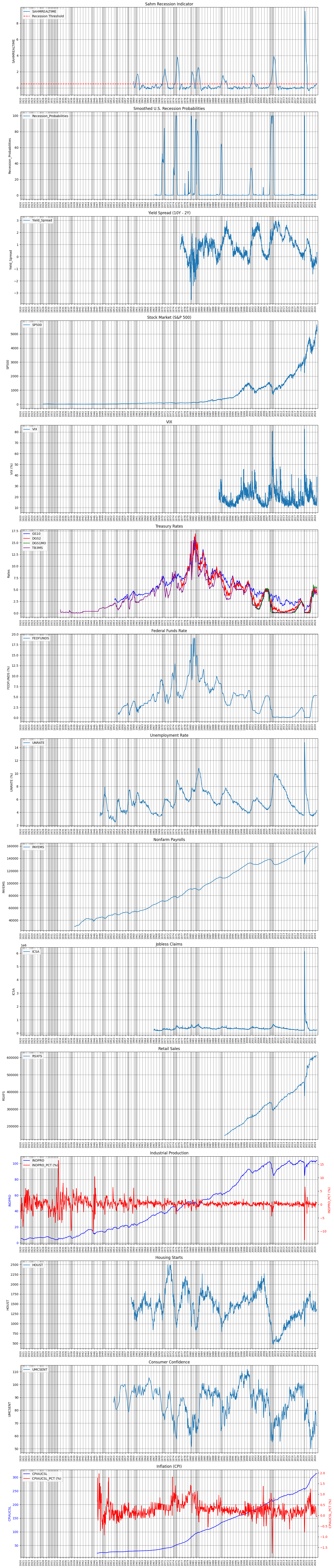
Figure. 1: Time-Series Analysis of Key Economic Indicators (1927-2024): The chart presents a timeline of critical economic metrics including the Sahm Recession Indicator, Smoothed U.S. Recession Probabilities, Yield Spread (10Y-2Y), S&P 500, VIX, Treasury Rates, Federal Funds Rate, Nonfarm Payrolls, Jobless Claims, Retail Sales, Industrial Production, Housing Starts, Consumer Confidence, and Inflation (CPI). The shaded regions indicate historical recessions.
Monitoring Key Recession Indicators
The Sahm indicator threshold has just been reached. Historically, this has been a reliable indicator, but even its creator acknowledges that ‘my recession rule can be broken‘.
This threshold alone does not confirm a current recession. It is important to continue monitoring this indicator to see if it rises to levels seen in 2020 or 2007.
Recession probabilities from NBER for 2024 have not yet spiked, which is a positive sign. However, ongoing monitoring of this probability is essential as the year progresses.
Yield Curve and Market Volatility Concerns
The yield curve presents a more concerning indicator. We observe a negative yield spread between 10-year and 2-year Treasury bonds, a classic warning sign. This reflects pessimism about future growth as investors demand higher yields for short-term bonds than for long-term ones.
The recent spike in the VIX also signals heightened market volatility and investor fear. This is troubling because it often triggers stock sell-offs, reducing market liquidity.
Economic Stability and Risks Ahead
Despite the recent massive sell-off in the S&P 500, the broader picture shows it is less significant than it might appear, as a sustained decline has not occurred. This suggests a normal market correction. Statistically, further downturns are expected.
While job openings remain stable, the slight rise in unemployment is concerning. Robust retail sales indicate strong consumer spending, but this may not last if economic pressures build. Declining housing starts and recent drops in consumer confidence are negative signs for the housing sector and broader economy.
Inflation and Recession Risks
High but stabilizing inflation indicates ongoing pressure that could strain the economy further if not controlled. Current indicators may not suggest a recession yet, but we are close or on the brink of one. Investors should prepare for continued economic challenges in the near term.
A Bloomberg article supports this view, discussing the rising risk of a U.S. recession despite recent optimism. It highlights statements from Federal Reserve Governor Christopher Waller and examines various economic indicators.
The article notes that while a “no-landing” scenario has been popular, recent data suggests potential economic weakness, making a recession more likely. It stresses the importance of preparing for this tail risk.
Additionally, the chart below shows the probability of a U.S. recession predicted by the Treasury spread, with a significant increase to 50% by April 2025. While this prediction does not indicate an immediate recession, it suggests we are close to one. Investors should take this data seriously, continue monitoring, and prepare for potential economic downturns in the coming year.
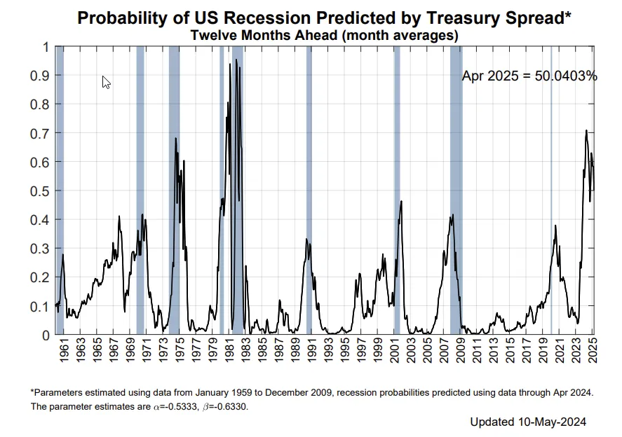
Figure. 3: Probability of Recession asn Predicted by Treasury Spreads (Source: Bloomberg).
2. History of Stock Market Decreases
It was the recent market drops which have sparked fear among investors and traders. This raised concerns about a prolonged market correction. To understand these declines’ significance and potential implications, we need to examine their historical context.
We will focus on the frequency of significant daily percentage declines in the S&P 500 index since the 1920s. This analysis will help determine whether the recent market downturn is a typical correction or a sign of a more significant economic shift.
We use historical data from the S&P 500 to calculate daily percentage changes in adjusted closing prices. The analysis sets thresholds for daily decreases (ranging from 1% to 10%) and counts the number of days each year the S&P 500 experienced declines exceeding these thresholds. We also annotate the data with recession periods to provide context.
					import yfinance as yf
import pandas as pd
import numpy as np
import matplotlib.pyplot as plt
import seaborn as sns

# Fetch historical data for S&P 500
sp500 = yf.download('^GSPC', start='1920-01-01')

# Calculate daily percentage change
sp500['Daily Change %'] = sp500['Adj Close'].pct_change() * 100

# Define the thresholds
thresholds = [1, 2, 3, 4, 5, 6, 7, 8, 9, 10]

# Initialize a dictionary to store the counts
counts = {f'>{threshold}%': [] for threshold in thresholds}

# Group by year and calculate counts
grouped = sp500.groupby(sp500.index.year)

for year, data in grouped:
    for threshold in thresholds:
        count = (data['Daily Change %'] < -threshold).sum()
        counts[f'>{threshold}%'].append(count)

# Create a DataFrame from the counts dictionary
counts_df = pd.DataFrame(counts, index=grouped.groups.keys())

# Convert crash periods to a DataFrame
crash_df = pd.DataFrame(list(crash_periods.items()), columns=['Start', 'End'])
crash_df['Start'] = pd.to_datetime(crash_df['Start'])
crash_df['End'] = pd.to_datetime(crash_df['End'])

# Function to check if a year had a recession
def is_recession(year):
    for _, row in crash_df.iterrows():
        if row['Start'].year <= year <= row['End'].year:
            return 'Recession'
    return 'No Recession'

# Apply the function to each year
counts_df['Recession'] = counts_df.index.map(is_recession)

# Apply color scale to the counts DataFrame
plt.figure(figsize=(15, 15))
sns.heatmap(counts_df.drop(columns='Recession'), cmap="Reds", annot=True, fmt="d", linewidths=.5, cbar_kws={'label': 'Count'})
plt.title('Number of Days with S&P 500 Decreases Exceeding Thresholds by Year', pad=20)
plt.xlabel('Thresholds')
plt.ylabel('Year')
plt.xticks(rotation=0)
plt.gca().xaxis.tick_top()
plt.gca().xaxis.set_label_position('top')

# Add recession labels to the y-axis
ax = plt.gca()
ax.set_yticks(np.arange(len(counts_df.index)) + 0.5)
y_labels = [f'{year:<4} {"( Recession  )" if recession == "Recession" else "(No Recession)":<13}' for year, recession in zip(counts_df.index, counts_df['Recession'])]
ax.set_yticklabels(y_labels, ha='right', fontfamily='monospace', fontsize=10, va='center')

plt.show()
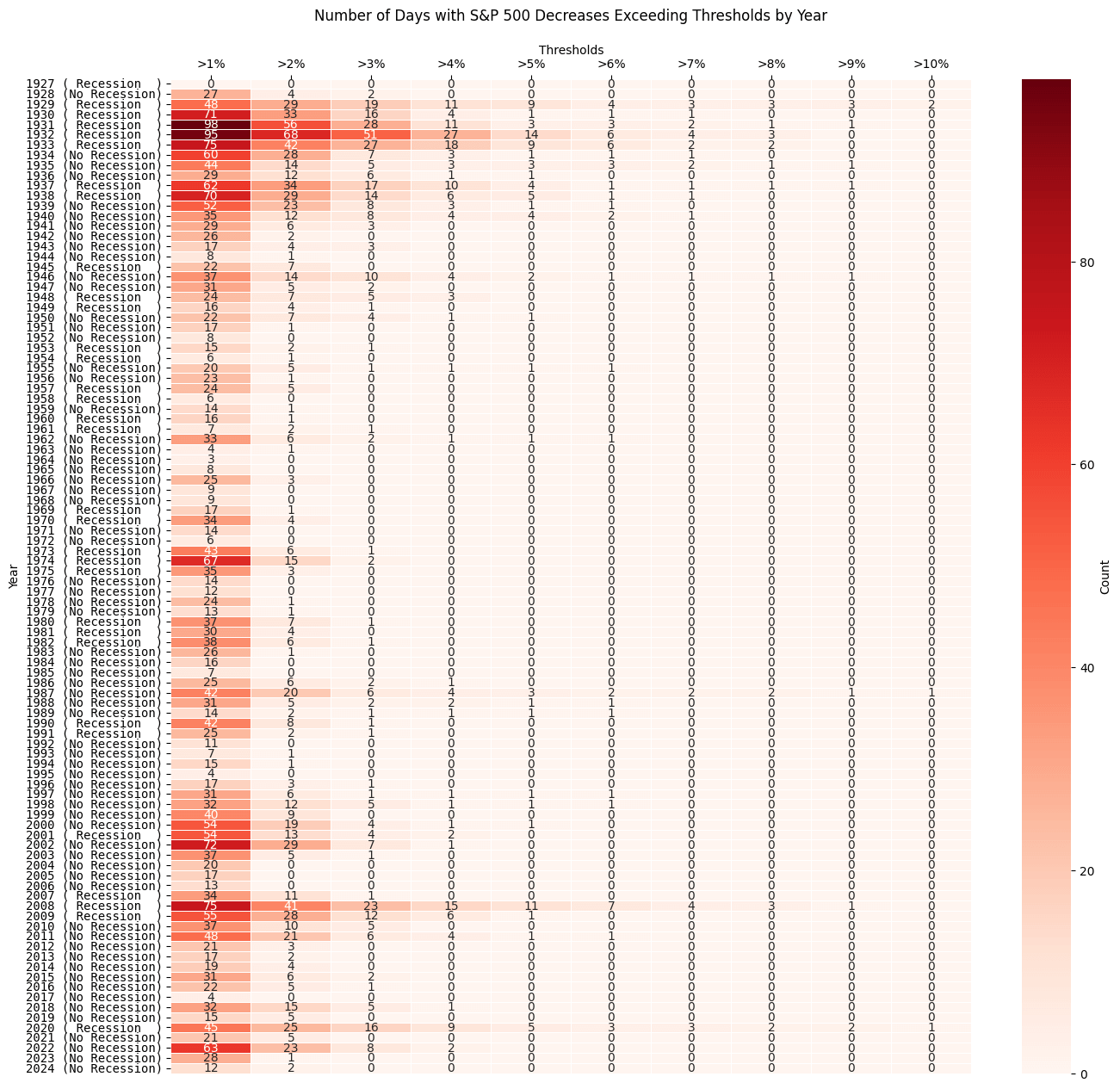
Figure. 2: Heatmap showing the number of days each year with S&P 500 daily percentage decreases exceeding thresholds from 1% to 10% since 1927. Years where recessions occured are further annotated.
In 2024, market declines exceeding 1% to 2% thresholds have occurred on several days. These drops indicate increased market volatility due to ongoing economic uncertainties like inflation concerns and geopolitical tensions.
Past recessions, such as the Great Recession (2008) and the COVID-19 pandemic (2020), saw sharp increases in market declines. 2024 has not reached those extreme patterns. The increasing frequency of market drops suggests investor wariness of potential economic slowdowns.
Future Projections and Risks
Statistically, more market declines would be expected in 2024, based on market drop frequencies in non-recessions, or “normal market conditions.” While current trends may seem alarming, they could still fall within typical market behavior patterns.
Investors should remain vigilant and avoid overreacting to short-term market movements. Focusing on broader economic indicators and long-term trends is crucial. Staying informed and maintaining a disciplined investment strategy will be key.
3. Treasury Yield Curve‘s Role in Recessions
The yield curve has been a reliable recession indicator of economic conditions and a strong predictor into the likelihood of a recession.
Let’s gather data to construct the yield curve over time, inspect spreads and explore its implications for economic growth and recession risk.
					import pandas as pd
import matplotlib.pyplot as plt
from pandas_datareader.data import get_data_fred
from datetime import datetime

# Define the start and end dates for the data
start_date = datetime(2023, 1, 1)  # Start date for data retrieval
end_date = datetime(2025, 6, 30)  # End date for data retrieval

# Retrieve the data for the yield curve
tickers = ['DGS1MO', 'DGS3MO', 'DGS6MO', 'DGS1', 'DGS2', 'DGS3', 'DGS5', 'DGS7', 'DGS10', 'DGS20', 'DGS30']
labels = {
    'DGS1MO': '1 Month',
    'DGS3MO': '3 Months',
    'DGS6MO': '6 Months',
    'DGS1': '1 Year',
    'DGS2': '2 Years',
    'DGS3': '3 Years',
    'DGS5': '5 Years',
    'DGS7': '7 Years',
    'DGS10': '10 Years',
    'DGS20': '20 Years',
    'DGS30': '30 Years'
}
# Fetch yield data from FRED for the specified tickers and date range
yield_data = get_data_fred(tickers, start=start_date, end=end_date)

# Drop rows with missing values to clean the data
yield_data = yield_data.dropna()

yield_data_copy = yield_data.copy()
3.1 Treasury Yield Over Time
Understanding how treasury yields change over time shows market expectations and potential economic trends. Specifically, we can interpret the yields over time in the following manner:
Decrease in short-term yields:
A decrease in short-term yields, such as the 1-month or 3-month Treasury yield, can indicate:
- Economic growth is slowing down.
- Investors are seeking safe-haven assets due to economic uncertainty.
- Example: If the 3-month Treasury yield falls from 1.5% to 1%, it may indicate that investors are becoming more cautious about the economy’s prospects.
Increase in long-term yields:
An increase in long-term yields, such as the 10-year or 30-year Treasury yield, can indicate:
- Economic growth and inflation expectations are increasing.
- Investors are demanding higher returns to compensate for rising inflation or economic uncertainty.
- Example: If the 10-year Treasury yield rises from 2% to 2.5%, it may indicate that investors expect stronger economic growth and higher inflation.
Contrasting yield movements:
A decrease in short-term yields and an increase in long-term yields can indicate:
- Economic uncertainty and rising inflation expectations.
- Investors are seeking safe-haven assets in the short-term, but expecting higher inflation and growth in the long-term.
- Example: If the 3-month Treasury yield falls from 1.5% to 1% and the 10-year Treasury yield rises from 2% to 2.5%, it may indicate that investors are uncertain about the economy’s prospects in the short-term, but expect higher inflation and growth in the long-term.
					yield_data = yield_data_copy

# Plot the time series for each term
plt.figure(figsize=(14, 8))
for ticker in tickers:
    plt.plot(yield_data.index, yield_data[ticker], label=labels[ticker])

plt.title('U.S. Treasury Yield Curve Time Series')  # Title of the plot
plt.xlabel('Date')  # X-axis label
plt.ylabel('Yield (%)')  # Y-axis label
plt.legend()  # Display legend
plt.grid(True)  # Show grid
plt.show()  # Display the plot

# Dynamic interpretation
max_yield = yield_data.max().max()  # Find the highest yield in the data
min_yield = yield_data.min().min()  # Find the lowest yield in the data
mean_yield = yield_data.mean().mean()  # Calculate the average yield

print(f"The highest yield observed in the time series is {max_yield:.2f}%.")
print(f"The lowest yield observed in the time series is {min_yield:.2f}%.")
print(f"The average yield across all maturities and dates is {mean_yield:.2f}%.")

# Interpretation based on the slope of the yield curve
# Calculate the difference between the longest and shortest maturity for each date
slope_indicator = yield_data['DGS30'] - yield_data['DGS1MO']
average_slope = slope_indicator.mean()  # Calculate the average slope

if average_slope > 0:
    print("On average, the yield curve shows an upward slope, which often indicates positive economic growth expectations.")
else:
    print("On average, the yield curve shows a downward slope, which may suggest a potential economic slowdown or recession.")

# Interpretation based on the trend
trend = yield_data.diff().mean()  # Calculate the average difference between consecutive yields
positive_trend_count = (trend > 0).sum()  # Count of positive trends
negative_trend_count = (trend < 0).sum()  # Count of negative trends

if positive_trend_count > negative_trend_count:
    print("Overall, yields are increasing over time, indicating rising interest rates.")
else:
    print("Overall, yields are decreasing over time, indicating falling interest rates.")
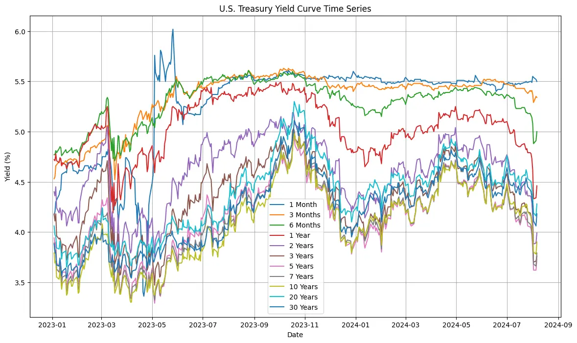
Figure. 4: Time series plot of U.S. Treasury yields for various maturities from January 2023 to July 2024.
Short-Term Yield Movements: Yields for short-term Treasuries (1 month, 3 months, 6 months) have shown fluctuations, especially around mid-2023. This volatility reflects changing market sentiments and adjustments to short-term economic expectations.
Long-Term Yield Stability: Long-term yields (10 years, 20 years, 30 years) have been more stable compared to short-term yields, but still show a gradual upward trend. This suggests that while short-term conditions may be volatile, long-term growth and inflation expectations are more stable and rising.
Inversion Periods: At times, yields on shorter-term Treasuries have exceeded those of longer-term ones, indicating an inverted yield curve. This inversion often signals investor concerns about potential economic downturns.
Sharp Drop and Rebound in July 2024: In July 2024, there was a sharp drop in yields across all maturities, followed by a quick rebound. This likely reflects a sudden market shock or heightened uncertainty, with the rebound indicating a swift market correction or intervention that restored some investor confidence.
3.2 Yield Spreads Over Time
Yield spreads measure the difference in yields between different Treasury securities. Yield spreads can tell us several things about the economy. For example:
- Economic uncertainty: High yield spreads indicate that investors are uncertain about the economy’s future prospects. For example, a 1% spread between 10-year and 2-year Treasury yields (2.5% vs. 1.5%) suggests that investors are demanding an additional 1% in yield to invest in a 10-year bond.
- Recession risk: Inverted yield spreads, such as a 10-year/2-year spread, can signal a recession. When the 10-year yield is lower than the 2-year yield (e.g., 2% vs. 2.5%), it indicates that investors expect short-term interest rates to rise, which can be a sign of economic slowdown.
- Inflation expectations: Yield spreads can also indicate inflation expectations. A high spread between 10-year and 2-year Treasury yields (e.g., 3% vs. 1.5%) suggests that investors expect inflation to rise in the future and are demanding higher yields for longer-term bonds.
- Monetary policy influence: The Federal Reserve’s interest rate decisions can impact yield spreads. For example, a 0.5% increase in the federal funds rate (from 1.5% to 2%) can cause the 10-year Treasury yield to rise from 2.5% to 3%, widening the yield spread and indicating economic uncertainty.
					import pandas as pd
import matplotlib.pyplot as plt

yield_data = yield_data_copy

# Calculate the spreads
spreads = pd.DataFrame({
    '10Y-2Y': yield_data['DGS10'] - yield_data['DGS2'],
    '10Y-3M': yield_data['DGS10'] - yield_data['DGS3MO'],
    '5Y-2Y': yield_data['DGS5'] - yield_data['DGS2'],
    '30Y-10Y': yield_data['DGS30'] - yield_data['DGS10'],
    '7Y-1Y': yield_data['DGS7'] - yield_data['DGS1'],
    '10Y-1Y': yield_data['DGS10'] - yield_data['DGS1']
})

# Plot the spreads over time
plt.figure(figsize=(14, 8))
for spread in spreads.columns:
    plt.plot(spreads.index, spreads[spread], label=spread)

plt.title('Yield Spreads Over Time')  # Title of the plot
plt.xlabel('Date')  # X-axis label
plt.ylabel('Spread (bps)')  # Y-axis label
plt.legend()  # Display legend
plt.grid(True)  # Show grid
plt.show()  # Display the plot

# Dynamic interpretation
spread_stats = spreads.describe()  # Get descriptive statistics for spreads

print("Spread Statistics:")
print(spread_stats)

for spread in spreads.columns:
    max_spread = spreads[spread].max()  # Maximum value of the spread
    min_spread = spreads[spread].min()  # Minimum value of the spread
    mean_spread = spreads[spread].mean()  # Mean value of the spread

    print(f"\nFor {spread}:")
    print(f"The highest spread observed is {max_spread:.2f} basis points.")
    print(f"The lowest spread observed is {min_spread:.2f} basis points.")
    print(f"The average spread over the period is {mean_spread:.2f} basis points.")

    if mean_spread > 0:
        print(f"On average, the {spread} spread is positive.")
        if spread in ['10Y-2Y', '10Y-3M']:
            print("This suggests that investors expect higher yields for longer-term bonds compared to shorter-term bonds, which is typical in a healthy, growing economy.")
        elif spread == '30Y-10Y':
            print("A positive 30Y-10Y spread indicates that long-term yields are higher than medium-term yields, reflecting stable long-term growth expectations.")
        else:
            print("Positive spreads here indicate that yields increase with maturity, reflecting investor confidence in steady economic growth.")
    else:
        print(f"On average, the {spread} spread is negative.")
        if spread in ['10Y-2Y', '10Y-3M']:
            print("This suggests that investors expect lower yields for longer-term bonds compared to shorter-term bonds, often seen as a warning sign of an impending recession. This is known as a yield inversion.")
        elif spread == '30Y-10Y':
            print("A negative 30Y-10Y spread suggests that long-term economic growth expectations are lower than medium-term expectations, potentially signaling long-term economic concerns. This can also indicate a yield inversion.")
        else:
            print("Negative spreads here indicate that yields decrease with maturity, reflecting investor pessimism about future economic conditions. This situation is also referred to as a yield inversion.")
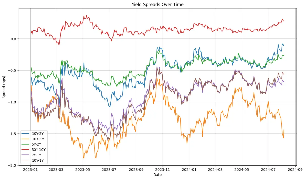
Figure. 5: Chart depicting the yield spreads over time from January 2023 to July 2024.
10Y-2Y and 10Y-3M Spreads: Both have been consistently negative. This indicates an inverted yield curve and potential economic recession.
Sharp Movements in Mid-2023: Significant drops in spreads occurred around mid-2023, followed by partial recoveries. These movements reflect market reactions to economic events or policy changes.
5Y-2Y and 30Y-10Y Spreads: These have been more stable. The 30Y-10Y spread remains positive, indicating some long-term growth expectations.
3.3 Yield Curve Over Time
The yield curve is a representation of the relationship between Treasury yields and their corresponding maturities. There are three main shapes by the yield curve which can be interpreted as follows:
Steepening yield curve:
A steepening yield curve, where long-term yields rise more than short-term yields, can indicate:
- Economic growth and inflation expectations are increasing.
- Investors are demanding higher returns to compensate for rising inflation or economic uncertainty.
- Example: If the 30-year Treasury yield rises from 3% to 3.5% and the 5-year Treasury yield remains at 2%, the yield curve steepens, it indicates that investors expect stronger economic growth and higher inflation.
Flattening yield curve:
A flattening yield curve, where long-term yields fall more than short-term yields, can indicate:
- Economic growth and inflation expectations are decreasing.
- Investors are seeking safe-haven assets due to economic uncertainty.
- Example: If the 10-year Treasury yield falls from 2.5% to 2% and the 1-year Treasury yield remains at 1.5%, the yield curve flattens, it indicates that investors are becoming more cautious about the economy’s prospects.
Inverted yield curve:
An inverted yield curve, where short-term yields exceed long-term yields, can indicate:
- Economic uncertainty and potential recession.
- Investors are seeking safe-haven assets due to economic uncertainty.
- Example: If the 6-month Treasury yield rises from 1.2% to 2.2% and the 20-year Treasury yield falls from 3.2% to 2.8%, the yield curve inverts, it indicates that investors are uncertain about the economy’s prospects and expect a potential recession.
					import pandas as pd
import plotly.express as px
import plotly.colors as pc

yield_data = yield_data_copy

# Sample labels dictionary
labels = {'DGS1MO': '1 Month', 'DGS3MO': '3 Months', 'DGS6MO': '6 Months', 'DGS1': '1 Year', 'DGS2': '2 Years', 'DGS5': '5 Years', 'DGS7': '7 Years', 'DGS10': '10 Years', 'DGS20': '20 Years', 'DGS30': '30 Years'}

# Function to prepare and plot yield curve data
def plot_yield_curve(yield_data, start_date):
    # Reset index to move DATE from index to column and rename it to 'DATE'
    yield_data.reset_index(inplace=True)
    yield_data.rename(columns={'index': 'DATE'}, inplace=True)

    # Convert DATE column to datetime format
    yield_data['DATE'] = pd.to_datetime(yield_data['DATE'])

    # Filter data based on the specified start date
    yield_data = yield_data[yield_data['DATE'] >= pd.to_datetime(start_date)]

    # Prepare data for Plotly
    yield_data_long = yield_data.melt(id_vars='DATE', var_name='Maturity', value_name='Yield')  # Transform data into long format

    # Ensure the 'Maturity' column is categorical and ordered
    yield_data_long['Maturity'] = pd.Categorical(yield_data_long['Maturity'], categories=list(labels.keys()), ordered=True)

    # Convert Yield to numeric to ensure proper plotting
    yield_data_long['Yield'] = pd.to_numeric(yield_data_long['Yield'])

    # Sort by date to ensure color scale represents the timeline
    yield_data_long.sort_values(['DATE', 'Maturity'], inplace=True)

    # Create a custom color sequence with a gradient from light to dark
    num_dates = yield_data_long['DATE'].nunique()
    color_scale = pc.sample_colorscale('Viridis', [n / num_dates for n in range(num_dates)])

    # Create an interactive plot with a custom color sequence
    fig = px.line(yield_data_long, x='Maturity', y='Yield', color='DATE',
                  title='Interactive U.S. Treasury Yield Curve',
                  labels={'Yield': 'Yield (%)', 'Maturity': 'Maturity'},
                  color_discrete_sequence=color_scale)

    # Update layout to enhance visualization
    fig.update_layout(
        xaxis=dict(
            tickvals=list(labels.keys()),
            ticktext=list(labels.values())
        )
    )

    fig.show()

    # Dynamic interpretation
    print("Dynamic Interpretation of Interactive U.S. Treasury Yield Curve:")

    # Analyzing the slope of the yield curve at various points
    slope_analysis = yield_data_long.groupby('DATE').apply(lambda df: df['Yield'].diff().mean())

    positive_slope_dates = slope_analysis[slope_analysis > 0].index
    negative_slope_dates = slope_analysis[slope_analysis < 0].index

    if len(positive_slope_dates) > len(negative_slope_dates):
        print("Most of the time, the yield curve has an upward slope, indicating positive economic growth expectations.")
    else:
        print("Most of the time, the yield curve has a downward slope, suggesting economic slowdown or recession concerns.")

    # Practical insights
    print("\nPractical Insights:")
    print("1. **Positive Slope (Normal Yield Curve)**: Indicates investor confidence in economic growth and rising interest rates. Long-term yields are higher than short-term yields.")
    print("2. **Negative Slope (Inverted Yield Curve)**: Often seen as a predictor of recession. Investors expect lower yields in the long term due to economic uncertainty or expected downturn.")
    print("3. **Flat or Humped Curve**: Indicates transitional phases in the economy. Investors may be uncertain about future growth or inflation.")

    # Summarize key observations
    print("\nKey Observations:")
    if len(positive_slope_dates) > 0:
        print(f"The yield curve was upward sloping on these dates: {positive_slope_dates[0]} to {positive_slope_dates[-1]}")
    if len(negative_slope_dates) > 0:
        print(f"The yield curve was downward sloping on these dates: {negative_slope_dates[0]} to {negative_slope_dates[-1]}")

# Fetch yield data from FRED for the specified tickers and date range
#yield_data = get_data_fred(tickers, start=start_date, end=end_date)

# Drop rows with missing values to clean the data
#yield_data = yield_data.dropna()

# Plot the data with a specified start date
plot_yield_curve(yield_data, '2024-06-01') # use start_date instead if you want the whole range
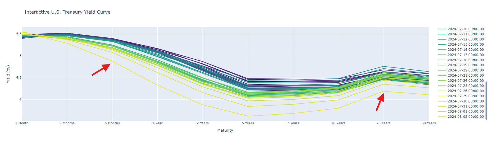
Figure. 6: Interactive visualization of the U.S. Treasury yield curve for various dates in July 2024.
The yield curve and yield spreads strongly indicate that the economy is very close to a recession one. Consistent inversion of key yield spreads (10Y-2Y, 10Y-3M) is a strong historical predictor of recessions. The flattening and inversion of the Treasury yield curve further reinforce this expectation.
3. Financial Analysts’ Take
As the market continues to fluctuate, top financial analysts from leading companies are sharing their insights on the potential for a recession. According to Scott Wren, senior global market strategist at Wells Fargo, “while recent economic indicators raise the risk of a recession, the odds of entering into one within the next 12 months are still low” (USA TODAY). This sentiment is echoed by Jan Hatzius, Chief Economist at Goldman Sachs, who notes that “the risk of a recession in the next 12 months is modestly higher” due to the recent market volatility and trade tensions (Yahoo Finance).
Meanwhile, Michael McDonough, Chief Economist at Bloomberg, is taking a more cautious approach, stating that “the recent market volatility is a wake-up call for investors, but it’s not necessarily a sign of a recession” (Bloomberg). Carl Riccadonna, Chief US Economist at Bloomberg, agrees, noting that “the yield curve inversion is a recession warning sign, but it’s not a guarantee of a recession” (Bloomberg).
At Morgan Stanley, Chetan Ahya, Chief Economist, is warning that the recent market volatility is a sign of a “late-cycle” economy, where growth is slowing, and risks are rising (CNBC). David Kelly, Chief Global Strategist at JPMorgan Funds, is advising investors to focus on high-quality stocks with strong balance sheets and stable earnings growth, as these companies are better equipped to weather a potential recession (Bloomberg).
UBS Global Wealth Management’s David Lefkowitz, head of US equities, is also optimistic, stating that the environment remains supportive for US equities and investors should have a full allocation to the asset class (Bloomberg). Deloitte Insights’ baseline forecast for the US economy remains hopeful, but they have also included a scenario that highlights the short-to-medium-term downside risks still clouding the outlook (Deloitte Insights).
Recession Fears Spark Global Market Slump
U.S. Economic Concerns
The recent market turmoil was triggered by a weaker-than-expected U.S. jobs report, with initial jobless claims rising significantly and the ISM manufacturing index signaling economic contraction at 46.8, below expectations of 48.8. This fueled fears of a slowing economy and prompted investors to anticipate potential emergency rate cuts by the Federal Reserve before their next meeting in September (The Economic Times).
The Fed’s decision in July not to lower interest rates added to concerns, and speculation around an emergency rate cut has created a divide among analysts, with some arguing it could prevent a deeper economic slump, while others believe it could signal panic and destabilize the market.(IC Markets) (WTVB).
Asian Markets Impact
The Japanese market experienced its worst day since 1987, with the Nikkei plummeting 12.4% due to recession fears and the Bank of Japan’s decision to raise interest rates. However, the market rebounded 10.2% the next day, clawing back some of its losses. The yen’s appreciation against the dollar played a crucial role in the turmoil, forcing traders to unwind their yen carry trades and sell off assets.
Despite the rebound, banks are still feeling the effects, and investors should remain cautious. The rapid unwinding of carry trades and concerns about a US recession have sent global markets into a tailspin, and it’s too early to conclude that the Japanese stock market has hit a bottom (WSJ).
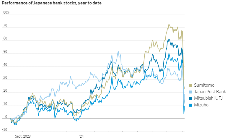
Figure. 7: Performance of Japanese Bank Stocks Year-to-Date. (Source: WSJ)
European and Emerging Markets
The global sell-off has also taken a toll on European stocks, with the DAX and CAC 40 plummeting to near six-month lows. Emerging markets have also been hit hard, with MSCI’s emerging market index down 4.1%. The perfect storm of US recession fears, poor tech earnings, and geopolitical tensions has created a toxic mix of uncertainty and fear in the markets. The yen’s appreciation against the dollar has added to the pressure, particularly on high-yielding emerging market currencies. As a result, investors are advised to exercise caution and be prepared for further market volatility.
Investor Sentiment and Market Outlook
Investor sentiment has been significantly impacted by recent market events. The CBOE Volatility Index (VIX) has surged above 20. This indicates more turbulence ahead. Despite this, some analysts, like Fundstrat’s Tom Lee, remain optimistic, seeing the current dip as a buying opportunity, particularly in sectors that have experienced significant pullbacks. The market has priced in a potential interest rate cut by the Federal Reserve, which could positively shift market sentiment and support a recovery in stock prices.
Others believe the recent employment report and market sell-off are not indicative of a looming recession, but rather a normal market correction following a prolonged bull run. The stability observed in corporate credit markets suggests that the underlying economic fundamentals remain relatively strong. Nevertheless, institutional sentiment is sending off mixed signals, with half expecting a recession and 60% projecting a soft landing as the most likely outcome. (Comerica, Business Insider Markets).
Factors Driving the Sell-Off
Several factors have contributed to the recent sell-off in U.S. markets:
- Economic Indicators: Weak economic indicators, such as a weaker-than-expected July jobs report.
- Federal Reserve Policy: The Federal Reserve’s decision not to lower interest rates in July has added to concerns about the economy, and there is growing debate about whether the Fed should implement an emergency rate cut.
- Global Economic Slowdown: The global economy has been slowing down, leading to concerns about the impact on corporate earnings and the stock market.
- Geopolitical Risks: Ongoing conflicts, such as the conflict in Ukraine, and trade tensions between the US and China have fueled uncertainty and increased volatility.
- Valuation Concerns: Some analysts have been warning that the stock market is overvalued, and that a correction is overdue.
- Yield Curve Inversion: The yield curve is inverted, which is often seen as a sign of a potential recession.
4. Topology Market Crashes
Topological data analysis (TDA), can help with detecting subtle patterns in complex data. Specifically, in the stock market, we can use TDA to identify potential crashes by analyzing the geometric changes in time series data.
Here we use a simple approach by computing the Wasserstein distance between persistent homology diagrams of log returns. This can be implemented using libraries such as Giotto-TDA and Ripser.
However, when using TDA to detect stock market crashes, one must consider the following practical aspects:
- Window size: Choose a suitable window size for computing the Wasserstein distance, as it can significantly impact the results.
- Threshold value: Set a reasonable threshold value to identify periods of high volatility and potential crashes.
- Interpretation: Be cautious when interpreting the results, as TDA is a descriptive tool and not a predictive one.
					import yfinance as yf
import numpy as np
from ripser import Rips
import persim
import matplotlib.pyplot as plt
import warnings

def fetch_data(ticker_name, start_date, end_date):
    """Fetch stock data from Yahoo Finance."""
    raw_data = yf.download(ticker_name, start=start_date, end=end_date)
    adjusted_close = raw_data['Adj Close'].dropna()
    prices = adjusted_close.values
    log_returns = np.log(prices[1:] / prices[:-1])
    return adjusted_close, log_returns

def compute_wasserstein_distances(log_returns, window_size, rips):
    """Compute the Wasserstein distances."""
    n = len(log_returns) - (2 * window_size) + 1
    distances = np.full((n, 1), np.nan)  # Using np.full with NaN values

    for i in range(n):
        segment1 = log_returns[i:i+window_size].reshape(-1, 1)
        segment2 = log_returns[i+window_size:i+(2*window_size)].reshape(-1, 1)

        if segment1.shape[0] != window_size or segment2.shape[0] != window_size:
            continue

        dgm1 = rips.fit_transform(segment1)
        dgm2 = rips.fit_transform(segment2)
        distance = persim.wasserstein(dgm1[0], dgm2[0], matching=False)
        distances[i] = distance

    return distances

def plot_data(prices, distances, threshold, window_size):
    """Generate the plots."""
    dates = prices.index[window_size:-window_size]
    valid_indices = ~np.isnan(distances)
    valid_dates = dates[valid_indices.flatten()]
    valid_distances = distances[valid_indices]

    alert_indices = [i for i, d in enumerate(valid_distances) if d > threshold]
    alert_dates = [valid_dates[i] for i in alert_indices]
    alert_values = [prices.iloc[i + window_size] for i in alert_indices]

    fig, ax = plt.subplots(2, 1, figsize=(25, 12), dpi=80)

    ax[0].plot(valid_dates, prices.iloc[window_size:-window_size], label=ticker_name)
    ax[0].scatter(alert_dates, alert_values, color='r', s=30)
    ax[0].set_title(f'{ticker_name} Prices Over Time')
    ax[0].set_ylabel('Price')
    ax[0].set_xlabel('Date')

    ax[1].plot(valid_dates, valid_distances)
    ax[1].set_title('Wasserstein Distances Over Time')
    ax[1].set_ylabel('Wasserstein Distance')
    ax[1].axhline(threshold, color='g', linestyle='--', alpha=0.7)
    ax[1].set_xlabel('Date')

    plt.tight_layout()
    plt.show()

# Configuration
ticker_name = '^GSPC' # SP500
start_date_string = "2015-01-01"
end_date_string = "2025-01-01"
window_size = 15
threshold = 0.04

warnings.filterwarnings('ignore')
prices, log_returns = fetch_data(ticker_name, start_date_string, end_date_string)
rips = Rips(maxdim=2)
wasserstein_dists = compute_wasserstein_distances(log_returns, window_size, rips)
plot_data(prices, wasserstein_dists, threshold, window_size)

Market volatility is rising, but Wasserstein distances remain below critical thresholds. This indicates stress without reaching crisis levels. The data does not conclusively indicate a recession but suggests increased caution. The S&P 500’s resilience and stable Wasserstein distances provide some reassurance.
Focusing on long-term investment horizons helps avoid panic selling during downturns. Overall, the analysis shows that while market volatility has increased, it is not yet at crisis levels. Investors should remain vigilant but cautious in their decisions.
All the analyses presentend here can be found in the following Google Colab Notebook:
Entreprenerdly - Assessing Key Economic Recession Indicators.ipynb
5. Discussion
Economic risks are rising, and the U.S. economy shows signs of slowing down. Although we are not necessarily in a recession now, caution is advised. The Sahm Recession Indicator has been triggered, but its significance remains debatable. Investors should monitor this closely.
Despite the current concerns, forecasts remain hopeful for 2024. Analysts predict that while the market may experience drops, these are likely to be normal corrections rather than signs of a deeper recession. Historical patterns support this view, which suggests that periodic downturns are part of typical market behavior.
Key Points to Consider
Rising Risks: Various indicators point to increasing economic risks. The global impact of economic slowdowns, particularly from major economies like China, contributes to this uncertainty.
Economic Slowdown: Current data suggests that the U.S. economy is decelerating. The yield curve, with its inverted key spreads like 10Y-2Y and 10Y-3M, signals potential recession. This inversion shows that investors expect lower growth.
Not in Recession Yet: The economy is not officially in a recession, but caution is warranted. Investors should pay attention to upcoming economic reports and indicators.
Hopeful Forecasts: Looking ahead to 2024, forecasts remain positive. While market corrections are expected, these are seen as standard adjustments rather than harbingers of a recession.
Market Drops and Corrections: Statistical analyses indicate that market drops are likely. However, these are attributed to normal market corrections rather than systemic issues.
Concluding Thoughts
The Federal Reserve’s stance on interest rates, geopolitical tensions, and economic data will play crucial roles in shaping the market’s direction.
Recommendations for Investors:
- Stay Informed: Keep up with the latest economic reports, Fed announcements, and geopolitical developments.
- Diversify Portfolios: Spread investments across various sectors and asset classes to mitigate recession risk.
- Evaluate Risk Tolerance: Conservative investors might shift assets into safer investments like high-quality bonds or TIPS.
- Increase cash reserves: Build up cash reserves to take advantage of potential investment opportunities during a recession.
- Reduce debt: Pay off high-interest debt and avoid taking on new debt to reduce financial stress during a recession.
- Long-term Perspective: Maintain a long-term investment perspective. Market corrections and volatility are part of the investment cycle.
Also worth reading:
Yield Data Retrieval, Curve Interpretation, Spreads, Correlations, and Regime Shifts
Predicting Market Crashes With Topology In Python
Modelling Extreme Stock Market Events With Copulas In Python

Newsletter