Estimating weighted portfolio beta, calculating FX conversion, and size index puts for dynamic drawdown protection
Sector tilts, concentrated bets, and currency exposures magnify losses when markets fall.
Simple diversification does not always account for the true market sensitivity, especially across borders.
During market crises, most asset correlations converge to 1. This is why you need to engineer an optimal portfolio hedge.
You must know the weighted beta of your entire portfolio and select the right instrument to mitigate losses in a downturn.
This article presents a practical, fully automated approach to estimate your real market risk, build a grid of hedge choices, and visualize the tradeoffs.
The complete Python notebook for the analysis is provided below.

Here, we’ll discuss the following topics:
- Automating the Hedging Analysis using Options
- Calculating Portfolio Beta accounting for FX
- Building a Hedge Options Metrics Grid
- Analyze Hedge Combinations and Pareto-Optimal Trades
- Measuring Coverage with Taylor Approximation
- Simulating Hedged vs. Unhedged Outcomes
1. Automating the Hedging Analysis using Options
Traditional portfolios rely on passive diversification to reduce risk. However, when markets fall sharply, correlations across assets spike.
Most positions begin to move together and erode the benefits of diversification.
Therefore, direct and systematic hedging becomes necessary to protect against large drawdowns.
Index put options are the standard tool for this job. They provide a defined payout when the market falls below a chosen level.
Unlike stop-losses or asset rotation, put options lock in protection for a known cost over a fixed period. An insurance, basically.
The key to effective hedging is matching the size of your hedge to the market risk your portfolio carries. This means:
- (i) Calculating your weighted portfolio beta to measure sensitivity to the market benchmark.
- (ii) Translating multi-currency positions into a common value base (e.g. from EUR to USD) to get the weights.
- (iii) Sizing index puts to cover the potential loss from a specific market move (e.g. 5% drop in 3 months).
The Hedging Workflow
The process starts by quantifying portfolio beta:

wi is the dollar (or base currency) weight and βi the beta of each asset relative to the market index.
With your beta exposure known, you can estimate the potential loss from a given market decline. For a portfolio value V and a market drop of x%:

You then match this risk using index puts, sized by their delta and contract multiplier:

Contracts needed, premium paid, and coverage at different drawdowns remain at the investor’s discretion.
Therefore, automating the process of exploring different strike prices, expiries, and hedge ratios is needed for quicker decisions.

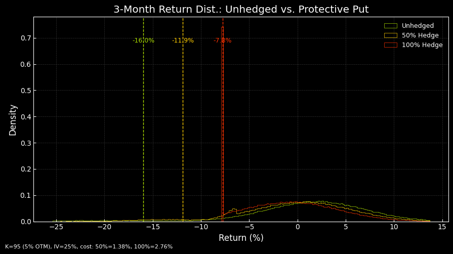
Figure 1. Hedged Portfolio vs Unhedged Portfolio Example. Distribution of 3-month portfolio returns comparing unhedged, 50% and 100% protective put hedges. Puts are 5% OTM, IV 25%, with VaR(5%) markers.
2. Calculating Portfolio Beta (Across FX)
2.1 Key Parameters
We set the key parameters in the script before starting the process.
First, we import the libraries:
					import pandas as pd
import numpy as np
import yfinance as yf
import math
from datetime import datetime
from dateutil.relativedelta import relativedelta
import matplotlib.pyplot as plt
import plotly.express as px
import plotly.graph_objects as go

# dark plotly
px.defaults.template = "plotly_dark"

# dark matplotlib
plt.style.use('dark_background')
Then, we list all individual holdings with ticker, currency, and market value.
We must also define the market benchmark index for beta calculations. Also, specify live FX tickers (from yfinance) to convert non-USD positions.
The example uses these settings:
- Five years of price history
- S&P 500 as benchmark
- Portfolio with US, European, and UK assets
- FX pairs for EUR and GBP
					# USER SETTINGS
BETA_YEARS = 5               # max history in years
INDEX_TKR  = "^GSPC"         # benchmark
MAPPING = [
    {"ticker": "VOO",      "value": 27_500.00, "ccy": "USD"},  # S&P 500 ETF (reduced, still core)
    {"ticker": "AMD",      "value": 13_500.00, "ccy": "USD"},  # Advanced Micro Devices (high beta, US semi)
    {"ticker": "AAPL",     "value": 11_000.00, "ccy": "USD"},  # Apple Inc.
    {"ticker": "TSLA",     "value": 10_000.00, "ccy": "USD"},  # Tesla Inc.
    {"ticker": "SHOP",     "value":  6_500.00, "ccy": "USD"},  # Shopify Inc. (US-listed, high beta tech)
    {"ticker": "ASML.AS",  "value":  7_000.00, "ccy": "EUR"},  # ASML Holding (EU tech, high beta)
    {"ticker": "ITM.L",    "value":  5_000.00, "ccy": "GBP"},  # ITM Power (UK growth/energy, high beta)
    {"ticker": "GLD",      "value":  4_500.00, "ccy": "USD"},  # SPDR Gold Shares (trimmed for risk)
    {"ticker": "EWZ",      "value":  5_000.00, "ccy": "USD"},  # iShares MSCI Brazil ETF (EM, high beta)
]
FX_TICKS = {"EUR": "EURUSD=X", "GBP": "GBPUSD=X"}
2.2 Get Data and Calculate Portfolio Beta
Now, we create a DataFrame from the portfolio mapping and download adjusted price history for all tickers, FX pairs, and the benchmark index.
Convert every holding into USD using latest FX rates. Calculate each position’s weight as a fraction of total USD value of the portfolio.
Rebuild price series for each security and adjust non-USD assets for spot FX. Compute daily returns for every position and the index.
Estimate beta for each security. If a beta is missing from yfinance, fall back to a rolling regression of returns against the index:

ri is the return of asset i, and rm is the return of the index.
Assign all betas back to the DataFrame. Calculate the weighted portfolio beta as the sum of each position’s beta times its weight (see formula above).

Newsletter