Identify and Trade Cointegrated Pairs
Pairs trading is a market-neutral trading strategy that involves matching a long position with a short position in two assets with a high correlation. This strategy aims to exploit relative price movements between the two assets, regardless of market direction. Using Python, you can automate the process of identifying cointegrated pairs, generating trading signals, and backtesting strategies.
In this article, we will guide you through identifying and trading cointegrated pairs. You’ll learn to detect these pairs, generate trading signals, and backtest the trading strategy. This guide includes an end-to-end implementation using Google Colab, making it accessible for both beginners and experienced algorithmic traders.
This article is structured as follows:
- Understanding Pairs Trading
- Pair Cointegration Detection
- Price Pairs Visualization
- Cointegration Tests
- Direction of the Relationship
- Buy and Sell Signals
- Trading Strategy P&L
1. Understanding Pairs Trading
1.1 What is Cointegration?
Cointegration refers to a statistical relationship between two or more time series, where their prices move together in the long run despite short-term deviations. In simpler terms, if two assets are cointegrated, their price spread will revert to a mean value over time.
1.2 Why Cointegration is Important
For pairs trading to be effective, the selected pairs need to be cointegrated rather than just correlated. Additionally, while correlation measures the strength and direction of a linear relationship between two variables, it does not account for the possibility that the relationship could diverge over time. Cointegration ensures that the relationship between the pairs remains stable in the long term.
1.3 Statistical Tests for Cointegration
Several statistical tests can be used to check for cointegration:
1.3.1 Engle-Granger Two-Step Method
The Engle-Granger method involves two steps and uses the Augmented Dickey-Fuller (ADF) test.
Step 1: Test for Stationarity
- First, apply the ADF test to each time series to check for the presence of a unit root. If the test rejects the null hypothesis, it indicates that the time series is stationary. For cointegration to exist, the individual series must be non-stationary in levels but stationary in their first differences.
Formula for the ADF Test:
Where:
- yt is the time series.
- Δyt is the first difference of yt.
- t is the time trend.
- ϵt is the white noise error term.
Step 2: Estimate the Cointegration Equation and Test Residuals
- Perform a linear regression of one series on the other (e.g., Yt on Xt) to obtain the residuals.
- Apply the ADF test to the residuals ϵt from this regression. If the residuals are stationary (rejecting the null hypothesis), it indicates that the series are cointegrated.
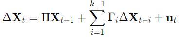
1.3.2 Johansen Cointegration Test
The Johansen test uses a vector autoregressive model to test the hypothesis of no cointegration against the alternative of cointegration among multiple time series.
Formula for the Johansen Test:
Where:
- Xt is a vector of the time series.
- ΔXt is the first difference of Xt.
- Π and Γi are coefficient matrices.
- ϵt is the white noise error term.
1.4 Implementing Pairs Trading Strategy
1. Identify Cointegrated Pairs: Use the ADF and Johansen tests to identify pairs of assets that are cointegrated.
2. Calculate the Spread: Once a pair is identified, calculate the spread between their prices.
3. Generate Trading Signals: Determine trading signals based on the z-score of the spread.

Where:
- μ is the mean of the spread.
- σ is the standard deviation of the spread.
4. Execute Trades:
- Go long on the spread (buy the first asset and sell the second) when the z-score is below a certain threshold.
- Go short on the spread (sell the first asset and buy the second) when the z-score is above a certain threshold.
5. Close Positions: Close the positions when the spread reverts to the mean (z-score returns to zero).
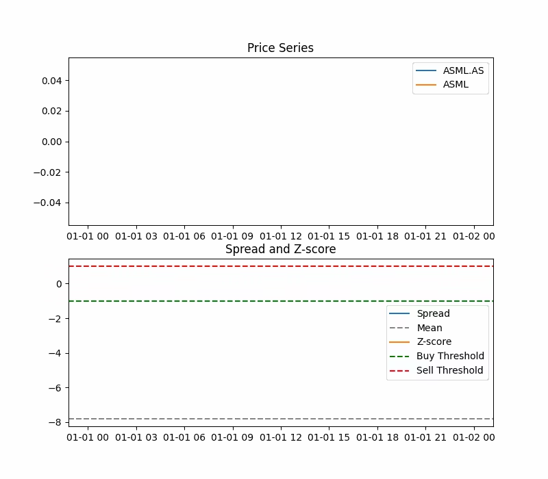
Figure. 1: Illustration of Pairs Trading: Taking Long and Short Positions in Cointegrated Assets to Profit from Relative Price Movements.
1.5 Extending the Strategy to Multiple Assets
In theory, pairs trading can be extended to three or more assets, often referred to as “triplets trading” or “multiple pairs trading.” The concept remains similar but involves more complex statistical methods to ensure cointegration among multiple assets.
1. Identify Cointegrated Groups: Use multivariate cointegration tests like the Johansen test to identify groups of assets that are cointegrated.
2. Calculate the Combined Spread: For three assets P1, P2, and P3, the combined spread could be calculated as:
Where β1 and β2 are hedge ratios obtained from multivariate regression.
3. Generate Trading Signals: Similar to the two-asset case, calculate the z-score of the spread and generate trading signals based on thresholds.
4. Execute and Manage Trades: Enter and exit positions based on the z-score, ensuring to balance the positions among all assets involved.
2. Preliminary Pair Cointegration Detection
We will identify possible cointegrated pairs preliminarily. This step helps select pairs from a universe of assets, especially when there is no prior knowledge of their relationship.
As previously mentioned, the Engle-Granger and Johansen tests are two primary methods used to detect cointegration for pairs trading. Let’s implement each of these methods.
Which Method is More Robust?
- Engle-Granger: Simpler and suitable for quick preliminary checks on pairs.
- Johansen: More robust for complex, multivariate analysis, providing deeper insights into cointegration among multiple assets.
2.1 Engle-Granger Cointegration Test
The Engle-Granger test involves two main steps: checking for stationarity and testing for cointegration.
The results are visualized in a heatmap, where darker colors indicate stronger cointegration relationships.
Limitations of Engle-Granger Test:
- Unidirectional: It assumes a single cointegrating relationship and may miss more complex interactions, such as for example lags and shifts.
- Two-Step Procedure: Errors in the first step (stationarity test) can propagate, affecting the second step.
- Single Pair: It only works for pairs of assets, not groups.
					import yfinance as yf
import pandas as pd
import numpy as np
import matplotlib.pyplot as plt
import seaborn as sns
from itertools import combinations
from statsmodels.tsa.stattools import coint

# Parameters
START_DATE = '2021-01-01'  # Start date for data collection
END_DATE = '2023-09-30'    # End date for data collection
P_VALUE_THRESHOLD = 0.05   # Threshold for cointegration p-value

# List of tickers for cryptocurrencies, bank stocks, and global indexes
crypto_tickers = ['BTC-USD', 'ETH-USD', 'BNB-USD', 'XRP-USD', 'ADA-USD', 'DOGE-USD', 'SOL-USD', 'DOT-USD']
stock_tickers = ['JPM', 'BAC', 'WFC', 'C', 'GS', 'MS', 'AAPL', 'AMZN', 'GOOGL', 'MSFT']
index_tickers = ['^DJI', '^IXIC', '^GSPC', '^FTSE', '^N225']

# Combine all tickers into one universe
universe_tickers = crypto_tickers + stock_tickers + index_tickers

# Function to load adjusted close price data for a given ticker
def load_ticker_ts_df(ticker, start, end):
    data = yf.download(ticker, start=start, end=end)  # Download data from Yahoo Finance
    return data['Adj Close']  # Return the adjusted close prices

# Load data for the universe of tickers
universe_tickers_ts_map = {ticker: load_ticker_ts_df(ticker, START_DATE, END_DATE) for ticker in universe_tickers}

# Function to sanitize the data
def sanitize_data(data_map):
    TS_DAYS_LENGTH = (pd.to_datetime(END_DATE) - pd.to_datetime(START_DATE)).days  # Total number of days in the date range
    data_sanitized = {}
    date_range = pd.date_range(start=START_DATE, end=END_DATE, freq='D')  # Create a date range
    for ticker, data in data_map.items():
        if data is None or len(data) < (TS_DAYS_LENGTH / 2):  # Skip if data is insufficient
            continue
        if len(data) > TS_DAYS_LENGTH:  # Trim data if it exceeds the required length
            data = data[-TS_DAYS_LENGTH:]
        data = data.reindex(date_range)  # Reindex data to match the date range
        data.replace([np.inf, -np.inf], np.nan, inplace=True)  # Replace infinities with NaN
        data.interpolate(method='linear', inplace=True)  # Interpolate missing values linearly
        data.fillna(method='pad', inplace=True)  # Forward fill remaining missing values
        data.fillna(method='bfill', inplace=True)  # Backward fill remaining missing values
        assert not np.any(np.isnan(data)) and not np.any(np.isinf(data))  # Ensure no NaNs or infinities remain
        data_sanitized[ticker] = data
    return data_sanitized

# Sanitize the data for all tickers
uts_sanitized = sanitize_data(universe_tickers_ts_map)

# Function to find cointegrated pairs
def find_cointegrated_pairs(tickers_ts_map, p_value_threshold=0.05):
    tickers = list(tickers_ts_map.keys())  # List of all tickers
    n = len(tickers)  # Number of tickers
    adj_close_data = np.column_stack([tickers_ts_map[ticker].values for ticker in tickers])  # Stack adjusted close prices column-wise
    pvalue_matrix = np.ones((n, n))  # Initialize p-value matrix with ones
    for i, j in combinations(range(n), 2):  # Iterate over all pairs of tickers
        result = coint(adj_close_data[:, i], adj_close_data[:, j])  # Perform cointegration test
        pvalue_matrix[i, j] = result[1]  # Store p-value
        pvalue_matrix[j, i] = result[1]  # Symmetric entry in the matrix
    pairs = [(tickers[i], tickers[j], pvalue_matrix[i, j]) for i in range(n) for j in range(i+1, n) if pvalue_matrix[i, j] < p_value_threshold]
    return pvalue_matrix, pairs  # Return the p-value matrix and list of cointegrated pairs

# Find cointegrated pairs and their p-values
pvalues, pairs = find_cointegrated_pairs(uts_sanitized, p_value_threshold=P_VALUE_THRESHOLD)

# Plot heatmap of p-values
plt.figure(figsize=(20, 20))
heatmap = sns.heatmap(pvalues, xticklabels=uts_sanitized.keys(), yticklabels=uts_sanitized.keys(), cmap='RdYlGn_r', mask=(pvalues > P_VALUE_THRESHOLD), linecolor='gray', linewidths=0.5)
heatmap.set_xticklabels(heatmap.get_xticklabels(), size=14, rotation=45)
heatmap.set_yticklabels(heatmap.get_yticklabels(), size=14)
plt.title('Cointegration Heatmap')
plt.show()

print("Heatmap for cointegrated pairs has been plotted.")
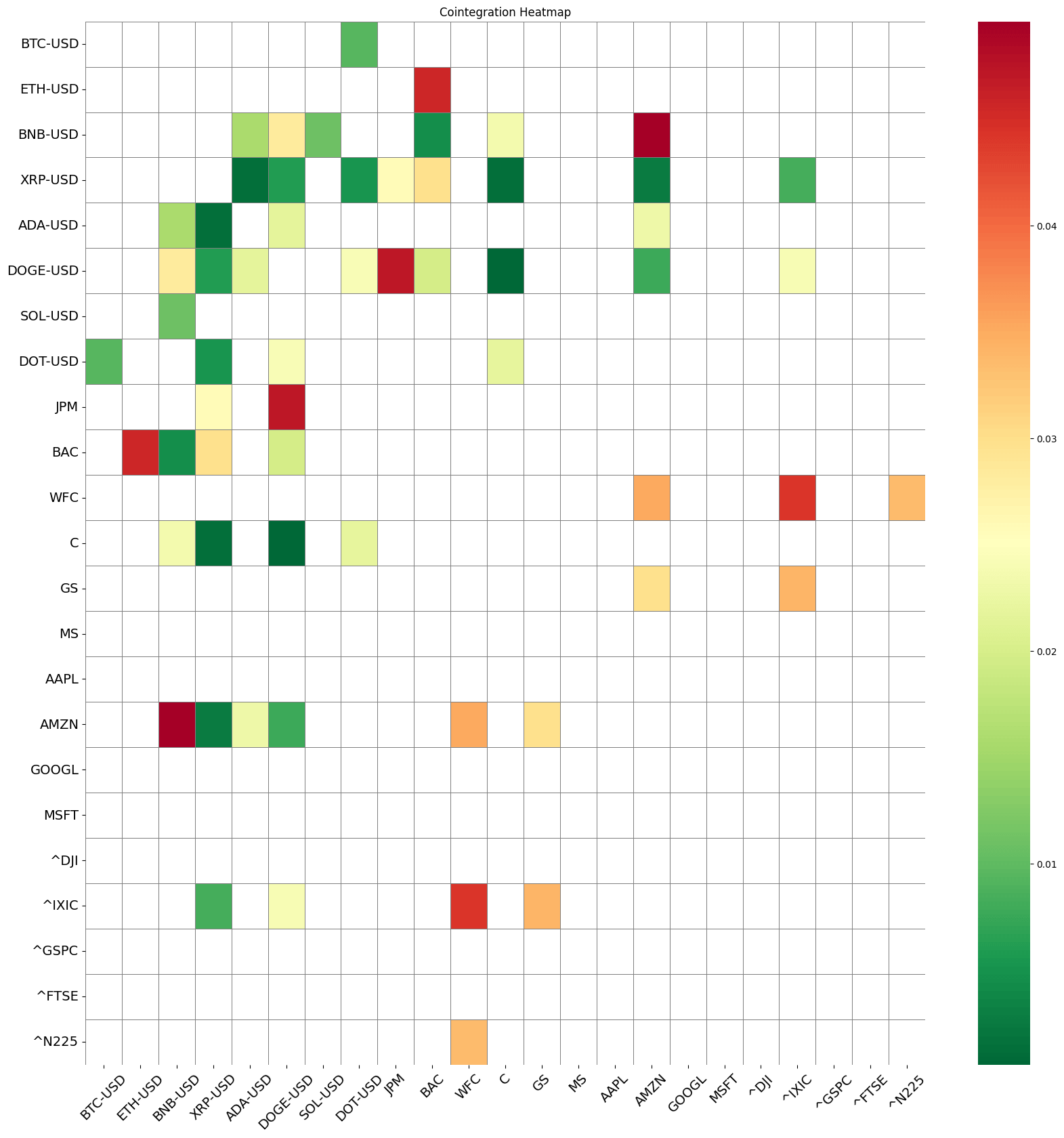
Figure. 2: Cointegration Heatmap: This heatmap visualizes the p-values of cointegration tests between various assets including cryptocurrencies, bank stocks, and global indexes. Darker colors indicate stronger cointegration relationships, highlighting potential pairs for trading strategies.
2.2 Johansen Cointegration Test
The Johansen test extends the Engle-Granger method by allowing for multiple cointegrating relationships among several time series. It uses a vector autoregressive model.
Data Preparation
- Load and sanitize data for a set of tickers.
- Ensure that data is continuous and free from missing values.
Perform Johansen Test
- Apply the Johansen test to the time series data.
- Identify cointegrated pairs based on the test statistics.
This method is particularly useful when dealing with multiple assets, as it can identify more complex cointegration structures.
Limitations of Johansen Test:
- Complexity: It is computationally more intensive and requires more sophisticated understanding.
- Parameter Sensitivity: Results can be sensitive to the chosen lag length and deterministic trend assumptions.
- Multiple Series: Suitable for analyzing more than two time series, which can be a strength or a complication.
					import yfinance as yf
import pandas as pd
import numpy as np
import matplotlib.pyplot as plt
import seaborn as sns
from itertools import combinations
from statsmodels.tsa.vector_ar.vecm import coint_johansen

# Parameters
START_DATE = '2021-01-01'  # Start date for data collection
END_DATE = '2023-09-30'    # End date for data collection
P_VALUE_THRESHOLD = 0.05   # Threshold for cointegration p-value
ROLLING_WINDOW_SIZE = 252  # Approximately one year of trading days
CONSISTENT_COINTEGRATION_THRESHOLD = 0.8  # 80% of the rolling windows

# List of tickers for cryptocurrencies, bank stocks, and global indexes
crypto_tickers = ['BTC-USD', 'ETH-USD', 'BNB-USD', 'XRP-USD', 'ADA-USD', 'DOGE-USD', 'SOL-USD', 'DOT-USD']
stock_tickers = ['JPM', 'BAC', 'WFC', 'C', 'GS', 'MS', 'AAPL', 'AMZN', 'GOOGL', 'MSFT']
index_tickers = ['^DJI', '^IXIC', '^GSPC', '^FTSE', '^N225']

# Combine all tickers into one universe
universe_tickers = crypto_tickers + stock_tickers + index_tickers

# Function to load adjusted close price data for a given ticker
def load_ticker_ts_df(ticker, start, end):
    data = yf.download(ticker, start=start, end=end)  # Download data from Yahoo Finance
    return data['Adj Close']  # Return the adjusted close prices

# Load data for the universe of tickers
universe_tickers_ts_map = {ticker: load_ticker_ts_df(ticker, START_DATE, END_DATE) for ticker in universe_tickers}

# Function to sanitize the data
def sanitize_data(data_map):
    TS_DAYS_LENGTH = (pd.to_datetime(END_DATE) - pd.to_datetime(START_DATE)).days  # Total number of days in the date range
    data_sanitized = {}
    date_range = pd.date_range(start=START_DATE, end=END_DATE, freq='D')  # Create a date range
    for ticker, data in data_map.items():
        if data is None or len(data) < (TS_DAYS_LENGTH / 2):  # Skip if data is insufficient
            continue
        if len(data) > TS_DAYS_LENGTH:  # Trim data if it exceeds the required length
            data = data[-TS_DAYS_LENGTH:]
        data = data.reindex(date_range)  # Reindex data to match the date range
        data.replace([np.inf, -np.inf], np.nan, inplace=True)  # Replace infinities with NaN
        data.interpolate(method='linear', inplace=True)  # Interpolate missing values linearly
        data.fillna(method='pad', inplace=True)  # Forward fill remaining missing values
        data.fillna(method='bfill', inplace=True)  # Backward fill remaining missing values
        assert not np.any(np.isnan(data)) and not np.any(np.isinf(data))  # Ensure no NaNs or infinities remain
        data_sanitized[ticker] = data
    return data_sanitized

# Sanitize the data for all tickers
uts_sanitized = sanitize_data(universe_tickers_ts_map)

# Function to perform Johansen test
def johansen_test(data, det_order=0, k_ar_diff=1):
    result = coint_johansen(data, det_order, k_ar_diff)
    return result.lr1, result.cvt

# Find cointegrated pairs using rolling windows
def find_cointegrated_pairs_rolling(tickers_ts_map, p_value_threshold=0.05, window_size=252, consistency_threshold=0.8):
    tickers = list(tickers_ts_map.keys())
    n = len(tickers)
    pvalue_matrix = np.ones((n, n))
    consistent_pairs = []

    for i, j in combinations(range(n), 2):
        pvalues = []
        for start in range(len(tickers_ts_map[tickers[i]]) - window_size + 1):
            end = start + window_size
            window_data_i = tickers_ts_map[tickers[i]].iloc[start:end]
            window_data_j = tickers_ts_map[tickers[j]].iloc[start:end]
            window_data = pd.concat([window_data_i, window_data_j], axis=1).dropna()
            if window_data.shape[0] < window_size:
                continue
            test_stat, crit_values = johansen_test(window_data)
            if test_stat[0] > crit_values[1, 1]:  # Using 95% critical value
                pvalues.append(0.01)  # Assign a small p-value if cointegrated
            else:
                pvalues.append(1)  # Assign a large p-value if not cointegrated

        pvalues = np.array(pvalues)
        consistent_cointegration = np.mean(pvalues < p_value_threshold)

        if consistent_cointegration >= consistency_threshold:
            consistent_pairs.append((tickers[i], tickers[j], consistent_cointegration))
            pvalue_matrix[i, j] = np.mean(pvalues)
            pvalue_matrix[j, i] = np.mean(pvalues)
        else:
            pvalue_matrix[i, j] = 1
            pvalue_matrix[j, i] = 1

    return pvalue_matrix, consistent_pairs

# Find cointegrated pairs and their p-values using rolling windows
pvalues, pairs = find_cointegrated_pairs_rolling(uts_sanitized, p_value_threshold=P_VALUE_THRESHOLD, window_size=ROLLING_WINDOW_SIZE, consistency_threshold=CONSISTENT_COINTEGRATION_THRESHOLD)

# Plot heatmap of p-values
plt.figure(figsize=(20, 20))
heatmap = sns.heatmap(pvalues, xticklabels=uts_sanitized.keys(), yticklabels=uts_sanitized.keys(), cmap='RdYlGn_r', mask=(pvalues > P_VALUE_THRESHOLD), linecolor='gray', linewidths=0.5)
heatmap.set_xticklabels(heatmap.get_xticklabels(), size=14, rotation=45)
heatmap.set_yticklabels(heatmap.get_yticklabels(), size=14)
plt.title('Cointegration Heatmap')
plt.show()

print("Heatmap for cointegrated pairs has been plotted.")
print(f"Identified Cointegrated Pairs (Consistency >= {CONSISTENT_COINTEGRATION_THRESHOLD*100}%):")
for pair in pairs:
    print(pair)

Figure. 3: Cointegration Heatmap: This heatmap displays the average p-values from rolling Johansen cointegration tests between various assets including cryptocurrencies, bank stocks, and global indexes. Darker colors represent stronger and more consistent cointegration relationships, highlighting potential pairs for trading strategies.
3. Visualize Price Pairs
Let’s visualize the prices series of the selected assets to understand the relationship between the assets.
3.1 Normalized Price Pairs
Normalization involves adjusting the price series to a common scale by subtracting the mean and dividing by the standard deviation.
Let’s start by getting the data for two selected stocks that we know to be cointegrated. In this example, we will use ASML, the ticker listed in the US, and ASML.AS, the ticker listed in the Netherlands.
					import warnings
warnings.filterwarnings('ignore')  # Ignore warnings for cleaner output
import yfinance as yf
import pandas as pd
import matplotlib.pyplot as plt

# Step 1: Data Collection
ticker1 = 'ASML.AS'  # Ticker for the first asset
ticker2 = 'ASML'     # Ticker for the second asset
start_date = '2022-01-01'  # Start date for data collection
end_date = '2023-09-30'    # End date for data collection

# Download the closing price data for each ticker within the specified date range
data1 = yf.download(ticker1, start=start_date, end=end_date)['Close']
data2 = yf.download(ticker2, start=start_date, end=end_date)['Close']

# Align the data on common dates to ensure they are comparable
aligned_data = pd.concat([data1, data2], axis=1, join='inner')  # Concatenate data on common dates
aligned_data.columns = [ticker1, ticker2]  # Rename columns to reflect ticker names
Next, we transform the price series and plot the results. This transformation helps in highlighting relative price movements and making it easier to spot trends and deviations.
					# Normalize the price series (subtract mean and divide by standard deviation)
normalized_data = (aligned_data - aligned_data.mean()) / aligned_data.std()
# This normalization transforms the data to have a mean of 0 and a standard deviation of 1.
# It allows us to compare the relative movements of the two stocks on the same scale.

# Plot the normalized price series of both stocks
plt.figure(figsize=(12, 6))  # Set the size of the plot
plt.plot(normalized_data[ticker1], label=f'Normalized {ticker1}')  # Plot normalized data for ticker1
plt.plot(normalized_data[ticker2], label=f'Normalized {ticker2}')  # Plot normalized data for ticker2
plt.title(f'Normalized Price Series for {ticker1} and {ticker2}')  # Add title to the plot
plt.xlabel('Date')  # Label for the x-axis
plt.ylabel('Normalized Price')  # Label for the y-axis
plt.legend()  # Add legend to the plot
plt.show()  # Display the plot

print(f"Normalized prices of {ticker1} and {ticker2} have been plotted. The plot shows how the two stocks have moved over time relative to their mean and standard deviation.")
# The print statement confirms that the normalized price series have been plotted.
# The plot helps visualize how the two stocks have moved relative to their historical averages.
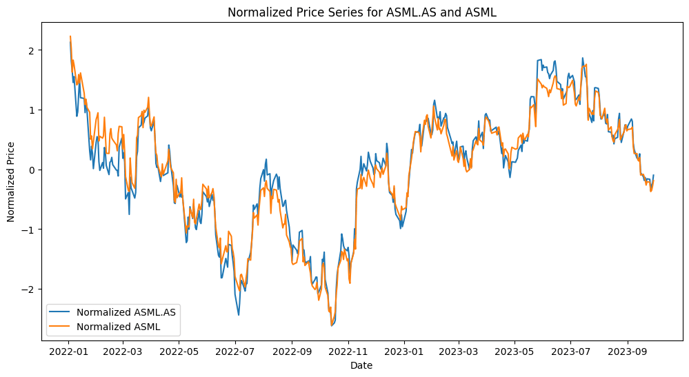
Figure. 4: Normalized Price Series for ASML.AS and ASML: This plot shows how the two stocks have moved over time relative to their mean and standard deviation.
3.2 Rolling Volatility
In pairs trading, assessing the volatility of the individual assets is important for several reasons:
- Risk Management: Higher volatility indicates higher risk. Understanding the volatility helps in setting appropriate stop-loss levels and managing the risk of the strategy.
- Entry and Exit Points: Changes in volatility can signal changes in market conditions, which might affect the timing of entry and exit points for the pairs trading strategy.
- Spread Volatility: Analyzing the rolling volatility of the spread between the two assets can also provide insights into the stability of their relationship and the likelihood of mean reversion.
					import numpy as np
# Calculate daily returns
returns = aligned_data.pct_change().dropna()

# Define the rolling window size (e.g., 30 days)
volatility_window = 30

# Calculate rolling volatilities (annualized)
volatility1 = returns[ticker1].rolling(volatility_window).std() * np.sqrt(252)
volatility2 = returns[ticker2].rolling(volatility_window).std() * np.sqrt(252)

# Plot the rolling volatilities
plt.figure(figsize=(10, 5))
plt.plot(volatility1, label=f"{ticker1} Volatility")
plt.plot(volatility2, label=f"{ticker2} Volatility")
plt.title(f"30-Day Rolling Historical Volatility for {ticker1} and {ticker2}")
plt.xlabel("Date")
plt.ylabel("Volatility")
plt.legend()
plt.show()

print(f"Rolling volatilities of {ticker1} and {ticker2} have been plotted. The plot shows the volatility of each stock over a 30-day window, annualized.")
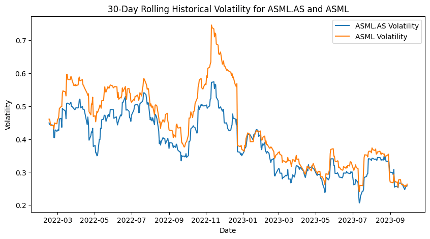
Figure. 5: 30-Day Rolling Historical Volatility for ASML.AS and ASML: This plot shows the annualized volatility of each stock over a 30-day window, illustrating their fluctuations and stability over time.
4. Cointegration Test with VECM
The Vector Error Correction Model (VECM) is a powerful tool for modeling long-term equilibrium relationships among cointegrated time series.
Unlike simple regression models, VECM accounts for both short-term dynamics and long-term relationships, making it particularly useful for pairs trading.
Steps in VECM Cointegration Testing
1. Check for Stationarity
- Use the Augmented Dickey-Fuller (ADF) test to check if the individual time series are stationary. Non-stationary time series with a unit root are necessary for cointegration analysis. If both series are stationary, there’s no need for cointegration analysis.
2. Perform Johansen Cointegration Test
- The Johansen test examines multiple time series for cointegration by using a vector autoregressive (VAR) model framework.
- It estimates the rank of cointegration (number of cointegrating relationships) and provides test statistics and critical values to determine cointegration.
3. Fit VECM
- VECM is an extension of VAR for cointegrated series. It separates short-term dynamics from long-term relationships using an error correction term.
- The model takes the form:
- where ΔXt is the differenced time series, Π contains the cointegration relations, Γi captures short-term effects, and ut is the error term.
- Π can be decomposed into αβ′, where α represents the speed of adjustment coefficients, and β contains the cointegrating vectors.
4. Analyze Residuals
- The residuals from the VECM should be stationary if the model is well specified. This indicates that the error correction mechanism is valid.
					import warnings
warnings.filterwarnings('ignore')  # Ignore warnings for cleaner output
import yfinance as yf
import pandas as pd
import numpy as np
import matplotlib.pyplot as plt
from statsmodels.tsa.api import VECM
from statsmodels.tsa.stattools import adfuller

# Check for stationarity of individual series using ADF test
adf_result1 = adfuller(aligned_data[ticker1])
adf_result2 = adfuller(aligned_data[ticker2])
# The adfuller function performs the Augmented Dickey-Fuller test
# It tests for a unit root in the time series and returns the test statistic and p-value

# Step 1: Perform Johansen cointegration test
from statsmodels.tsa.vector_ar.vecm import coint_johansen

def johansen_test(data, det_order=0, k_ar_diff=1):
    result = coint_johansen(data, det_order, k_ar_diff)
    return result.lr1, result.cvt
# The johansen_test function performs the Johansen cointegration test
# It returns the test statistics and critical values for cointegration

coint_test_stat, coint_critical_values = johansen_test(aligned_data)
# Apply the Johansen test on the aligned data to check for cointegration

# Step 2: If cointegration exists, proceed with VECM
vecm = VECM(aligned_data, k_ar_diff=1, coint_rank=1)
vecm_fit = vecm.fit()
# The VECM (Vector Error Correction Model) is fitted to the data if cointegration exists
# k_ar_diff is the number of lags and coint_rank is the cointegration rank

# Analyzing the residuals for stationarity
residuals = vecm_fit.resid
adf_residuals_1 = adfuller(residuals[:, 0])
adf_residuals_2 = adfuller(residuals[:, 1])
# The residuals from the VECM model are tested for stationarity using the ADF test

# Creating a DataFrame for residuals
residuals_df = pd.DataFrame(residuals, columns=[f'Residual_{ticker1}', f'Residual_{ticker2}'])
# Create a DataFrame to store the residuals for better visualization and analysis

# Plotting the residuals
plt.figure(figsize=(12, 6))
plt.plot(residuals_df, label=['Residual ASML.AS', 'Residual ASML'])
plt.axhline(0, color='red', linestyle='--', label='Zero Line')
plt.title('Residuals from VECM')
plt.xlabel('Date')
plt.ylabel('Residuals')
plt.legend()
plt.show()
# Plot the residuals to visualize their behavior over time
# The red line at y=0 helps identify deviations from the mean

# Print Statements to show ADF test results
print(f"ADF Statistic for {ticker1}: {adf_result1[0]}")
print(f"p-value for {ticker1}: {adf_result1[1]}")
print(f"ADF Statistic for {ticker2}: {adf_result2[0]}")
print(f"p-value for {ticker2}: {adf_result2[1]}")

# Interpretation of ADF results
if adf_result1[1] < 0.05:
    print(f"{ticker1} is stationary.")
else:
    print(f"{ticker1} is not stationary.")

if adf_result2[1] < 0.05:
    print(f"{ticker2} is stationary.")
else:
    print(f"{ticker2} is not stationary.")
# Interpretation of the ADF test results for each ticker
# A p-value less than 0.05 indicates stationarity

print(f"Cointegration Test Statistics: {coint_test_stat}")
print(f"Critical Values (90%, 95%, 99%): {coint_critical_values}")
# Print the test statistics and critical values from the Johansen cointegration test

# Summary of the VECM model (optional)
# print(vecm_fit.summary())

# Interpretation of Johansen test results
if coint_test_stat[0] > coint_critical_values[0, 1]:
    print(f"The two stocks {ticker1} and {ticker2} are cointegrated.")
else:
    print(f"The two stocks {ticker1} and {ticker2} are not cointegrated.")
# Check if the test statistic is greater than the critical value at the 95% confidence level
# If so, the stocks are cointegrated

print(f"ADF Statistic for VECM residuals of {ticker1}: {adf_residuals_1[0]}")
print(f"p-value for VECM residuals of {ticker1}: {adf_residuals_1[1]}")
print(f"ADF Statistic for VECM residuals of {ticker2}: {adf_residuals_2[0]}")
print(f"p-value for VECM residuals of {ticker2}: {adf_residuals_2[1]}")
# Print the ADF test results for the residuals from the VECM model

# Interpretation of VECM residuals
if adf_residuals_1[1] < 0.1:
    print(f"The residuals of the VECM model for {ticker1} are stationary, confirming cointegration.")
else:
    print(f"The residuals of the VECM model for {ticker1} are not stationary, suggesting no cointegration.")

if adf_residuals_2[1] < 0.1:
    print(f"The residuals of the VECM model for {ticker2} are stationary, confirming cointegration.")
else:
    print(f"The residuals of the VECM model for {ticker2} are not stationary, suggesting no cointegration.")
# Interpretation of the stationarity of the residuals from the VECM model
# A p-value less than 0.1 indicates stationarity, confirming cointegration

# Creating a table for Johansen test results
johansen_results = pd.DataFrame({
    'Test Statistic': coint_test_stat,
    '90% Critical Value': coint_critical_values[:, 0],
    '95% Critical Value': coint_critical_values[:, 1],
    '99% Critical Value': coint_critical_values[:, 2]
}, index=[f'Cointegration Test {i+1}' for i in range(len(coint_test_stat))])

print("\nJohansen Cointegration Test Results:\n")
print(johansen_results)
# Create a DataFrame to neatly display the Johansen test results with their critical values

# Comprehensive Interpretation

# ADF Test Results
print("\nADF Test Results Interpretation:")
if adf_result1[1] < 0.05:
    print(f"{ticker1} is stationary, indicating the series does not have a unit root.")
else:
    print(f"{ticker1} is not stationary, indicating the series has a unit root.")

if adf_result2[1] < 0.05:
    print(f"{ticker2} is stationary, indicating the series does not have a unit root.")
else:
    print(f"{ticker2} is not stationary, indicating the series has a unit root.")
# Detailed interpretation of the ADF test results for each ticker

# Johansen Cointegration Test Results
print("\nJohansen Cointegration Test Results Interpretation:")
if coint_test_stat[0] > coint_critical_values[0, 1]:
    print(f"The two stocks {ticker1} and {ticker2} are cointegrated at the 95% confidence level.")
else:
    print(f"The two stocks {ticker1} and {ticker2} are not cointegrated at the 95% confidence level.")
# Detailed interpretation of the Johansen test results

# VECM Residuals Stationarity Test Results
print("\nVECM Residuals Stationarity Test Results Interpretation:")
if adf_residuals_1[1] < 0.1:
    print(f"The residuals of the VECM model for {ticker1} are stationary, confirming cointegration.")
else:
    print(f"The residuals of the VECM model for {ticker1} are not stationary, suggesting no cointegration.")

if adf_residuals_2[1] < 0.1:
    print(f"The residuals of the VECM model for {ticker2} are stationary, confirming cointegration.")
else:
    print(f"The residuals of the VECM model for {ticker2} are not stationary, suggesting no cointegration.")
# Detailed interpretation of the VECM residuals' stationarity test results
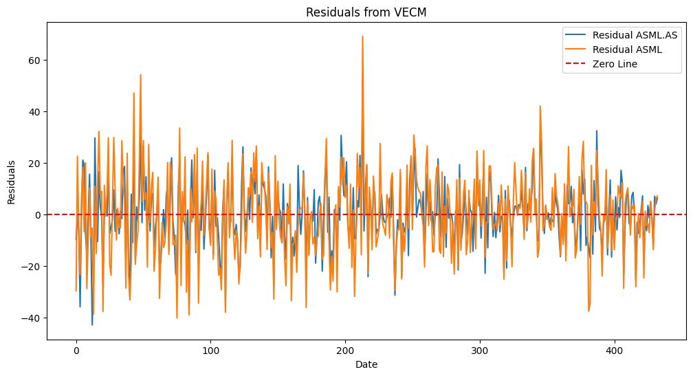
Figure. 6: Residuals from VECM: This plot shows the residuals of the Vector Error Correction Model (VECM) for ASML.AS and ASML, indicating stationarity around the zero line and confirming cointegration between the two stocks.
					ADF Statistic for ASML.AS: -2.7412180351995725
p-value for ASML.AS: 0.06717326704560742
ADF Statistic for ASML: -2.5972778964553966
p-value for ASML: 0.0935611770502971
ASML.AS is not stationary.
ASML is not stationary.
Cointegration Test Statistics: [32.73840264  6.33200307]
Critical Values (90%, 95%, 99%): [[13.4294 15.4943 19.9349]
 [ 2.7055  3.8415  6.6349]]
The two stocks ASML.AS and ASML are cointegrated.
ADF Statistic for VECM residuals of ASML.AS: -21.75268965443752
p-value for VECM residuals of ASML.AS: 0.0
ADF Statistic for VECM residuals of ASML: -20.854770789640124
p-value for VECM residuals of ASML: 0.0
The residuals of the VECM model for ASML.AS are stationary, confirming cointegration.
The residuals of the VECM model for ASML are stationary, confirming cointegration.

Johansen Cointegration Test Results:

                      Test Statistic  90% Critical Value  95% Critical Value  \
Cointegration Test 1       32.738403             13.4294             15.4943
Cointegration Test 2        6.332003              2.7055              3.8415

                      99% Critical Value
Cointegration Test 1             19.9349
Cointegration Test 2              6.6349

ADF Test Results Interpretation:
ASML.AS is not stationary, indicating the series has a unit root.
ASML is not stationary, indicating the series has a unit root.

Johansen Cointegration Test Results Interpretation:
The two stocks ASML.AS and ASML are cointegrated at the 95% confidence level.

VECM Residuals Stationarity Test Results Interpretation:
The residuals of the VECM model for ASML.AS are stationary, confirming cointegration.
The residuals of the VECM model for ASML are stationary, confirming cointegration.
5. Identify Direction of the Relationship
Understanding the direction of the relationship between cointegrated pairs is needed for generating trading signals in pairs trading.
This section delves into methods like cross-correlation and Granger causality to determine lead-lag relationships between assets.
5.1 Cross-Correlation
Cross-correlation measures the similarity between two time series at different lags. This helps identify which asset tends to lead or lag the other, providing insights into the timing of trades.
Steps for Cross-Correlation Analysis:
1. Calculate Cross-Correlation:
- Compute the cross-correlation between the returns of two assets over a range of lags. This shows how the movement of one asset relates to the movement of the other at various time intervals.
- Positive lag values indicate that the first asset leads the second asset, while negative lag values indicate the opposite.
2. Identify Peaks:
- Peaks in the cross-correlation plot indicate the lags at which the correlation is strongest. These peaks help determine the lead-lag relationship between the assets.
The cross_correlation function below calculates the correlation between two series at different lags. If the lag is positive, it correlates the series1 values at time t with series2 values at time t+lag. If negative, it correlates series1 values at time t with series2 values at time t-lag.
Also worth reading:
Bootstrapping Future Price Movements Probabilities

Newsletter